Harnessing AI for Better Health:
An Introduction to Health Scan Innovation
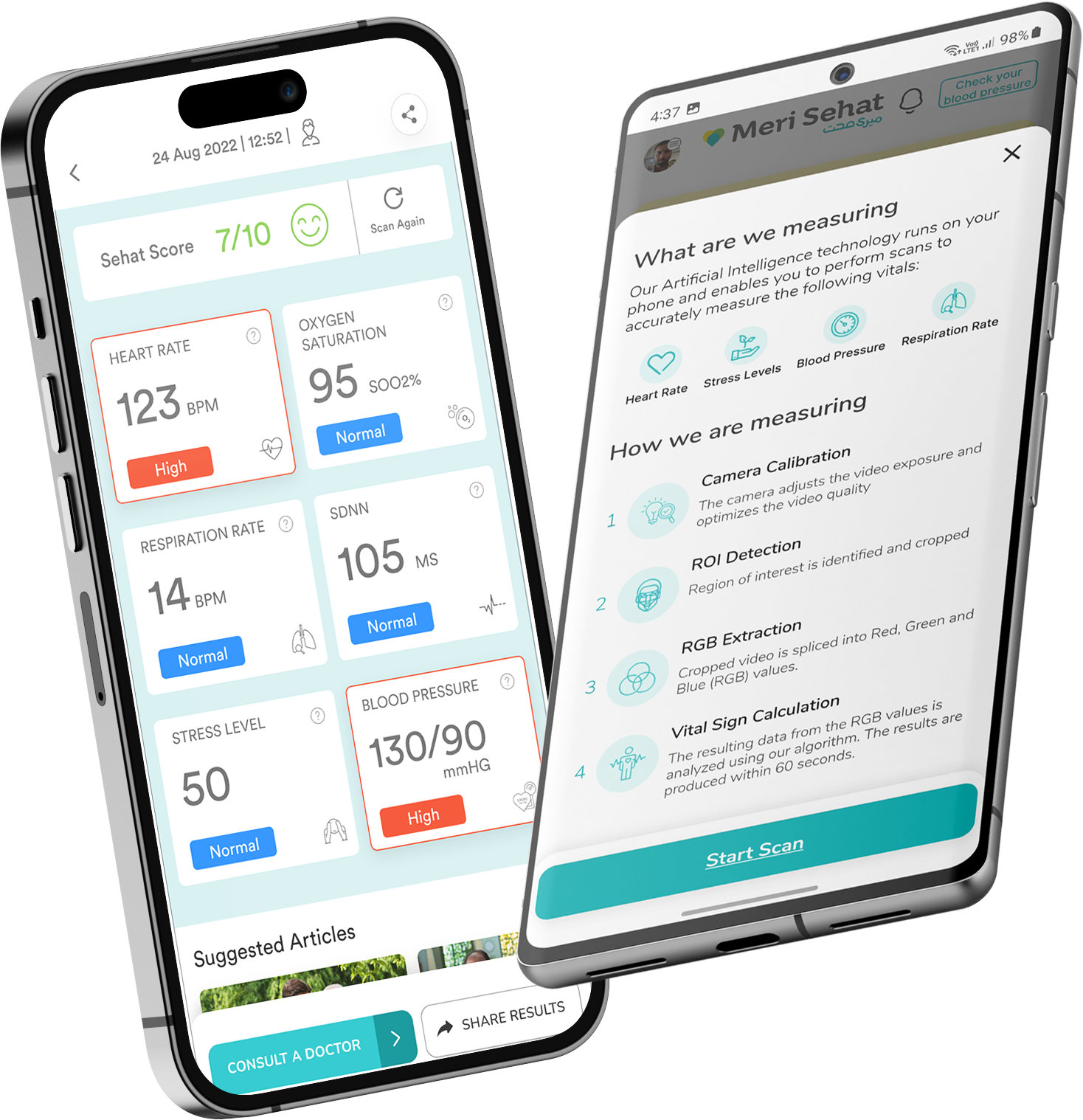
Our AI-driven Vital Monitoring Platform securely tracks crucial health metrics, including heart rate, blood pressure, stress levels, oxygen saturation, heart rate variability, and pulse rate quotient, offering comprehensive, software-only health management solutions for users.
(rPPG) Artificial Intelligence at Work
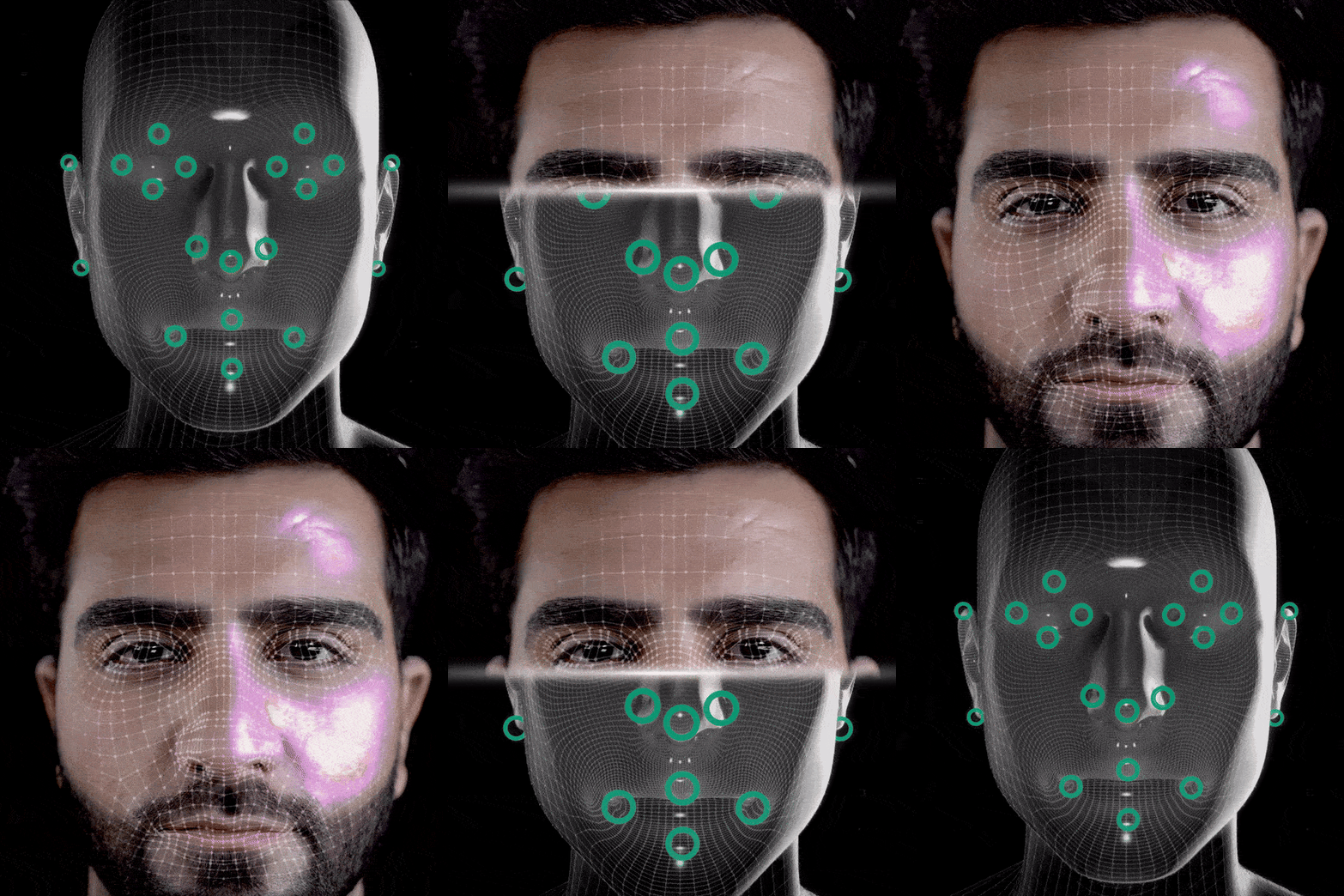
Remote photoplethysmography (rPPG) is a technology that uses video images to measure
changes in blood flow and blood volume in the microvascular bed of the skin.
(rPPG) Artificial Intelligence at Work
Remote photoplethysmography (rPPG) is a technology that uses video images to measure
changes in blood flow and blood volume in the microvascular bed of the skin.
Remote photoplethysmography (rPPG) is a technology that uses video images to measure changes in blood flow and blood volume in the microvascular bed of the skin.
  • Heart rate: rPPG can be used to measure the frequency of blood flow in the microvasculature of the skin, which can provide an estimate of heart rate.
  • Respiration rate: rPPG detects changes in blood flow and blood volume associated with respiration, allowing it to be used as a measure of respiration rate.
  • Blood pressure: rPPG measures blood pressure by analyzing changes in blood volume through light absorption, typically using a camera to detect subtle variations in skin color caused by pulsatile blood flow.
  • Oxygen saturation: rPPG measures changes in blood flow and blood volume associated with oxygenation and deoxygenation, allowing it to be used as a measure of oxygen saturation.
  • Heart rate: rPPG can be used to measure the frequency of blood flow in the microvasculature of the skin, which can provide an estimate of heart rate.
  • Respiration rate: rPPG may be able to detect changes in blood flow and blood volume associated with respiration, allowing it to be used as a measure of respiration rate.
  • Blood pressure: Some studies have suggested that rPPG may be able to provide estimates of blood pressure, although more research is needed to understand the accuracy and reliability of this application.
  • Oxygen saturation: rPPG may be able to measure changes in blood flow and blood volume associated with oxygenation and deoxygenation, allowing it to be used as a measure of oxygen saturation.
Back Channel Machine Learning
Remote photoplethysmography (rPPG) monitors change in color and time interval between the changes
are calculated toget the vital signs such as heart rate, heart rate variability and respiration rate:

Remote photoplethysmography (rPPG) monitors change in color and time interval between the changes are calculated toget the vital signs such as heart rate, heart rate variability and respiration rate:

Image acquisition

Capturing video images with a high-spec camera or similar imaging device is integral, as the accuracy and reliability of rPPG measurements can be significantly influenced by the quality and resolution of these images.
Install Meri Sehat on Android

Preprocessing

The correction and enhancement of video images improves their clarity and quality. This process includes various techniques, including noise reduction, illumination correction, and color correction.
Install Meri Sehat on iOS

Signal processing

The extracted features from the signal are analysed and interpreted to obtain information about the changes in blood flow and volume. This involves using techniques like filtering, feature selection, and statistical analysis.
Install Meri Sehat on Android

Region of interest (ROI) selection

The region of the skin is identified that will be analyzed by rPPG. This involves selecting the ROI based on various factors such as the visibility of blood vessels, skin color, or other characteristics.
Install Meri Sehat on iOS

Feature extraction

Extracting key data from the video images that are related to the changes in blood flow and volume. These include information about the intensity, texture, and spatial distribution of the pixels in the ROI.
Install Meri Sehat on Android

Vital sign estimation

Physiological parameters like heart rate, respiration rate, and blood pressure are estimated based on rPPG signals. This is done using algorithms trained on data collected from previous rPPG measurements.
Install Meri Sehat on iOS

rPPG algorithms & statistical models

  • Principal component analysis (PCA) reduces data dimensionality, extracting crucial features from datasets, simplifying rPPG signal analysis.
  • Support vector machine (SVM) is a classification algorithm that categorizes rPPG signals based on parameters like heart rate.
  • Decision trees model decisions using dataset characteristics, identifying rPPG signal patterns and predicting physiological parameters.
  • Linear regression models relationships between a dependent variable and independent ones. It estimates parameters like heart rate from rPPG signals.

What are ANNs?

ANNs comprise interconnected nodes in layers: input, hidden, and output. Each node processes input using an activation function, providing an output. During learning, connection weights are adjusted to reduce prediction error.

Artificial Neural Networks (ANNs) are computational models resembling the structure and function of biological brain networks. They process, learn from, and identify complex patterns in data, useful for artificial intelligence tasks.

ANNs use algorithms like backpropagation to understand data relationships. They're utilized in tasks such as image recognition, language processing, and speech recognition.

ANN Benchmark and standards

  • Robustness: Evaluates the ANN's ability to handle video image variations. Metrics may include sensitivity to changes in lighting and background.
  • Generalization: Assesses the ANN's ability to apply its knowledge to new data, comparing its performance to other models on unseen datasets.
  • Efficiency: Measures the ANN's computational and storage requirements, assessing scalability using metrics like training time and memory requirements.
  • Accuracy: Measures the ANN's prediction of physiological quantities from video images, assessed through metrics like mean absolute error (MAE) and correlation coefficients.
The first remote vital monitoring tool.

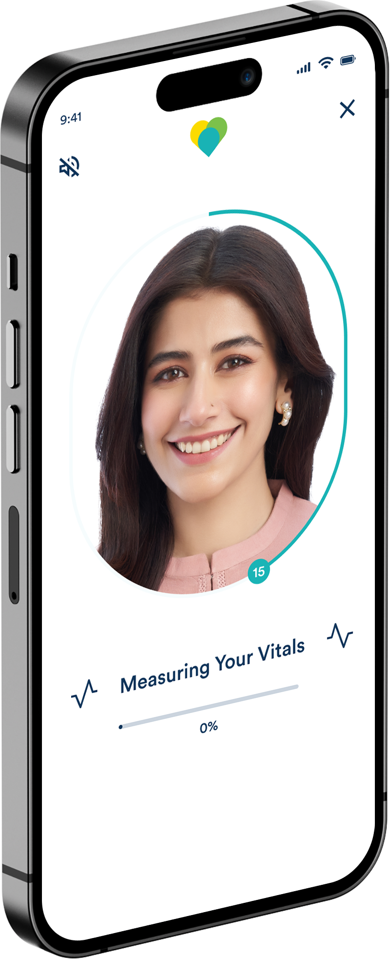
Experience the freedom of taking blood pressure readings anytime, anywhere with the Meri Sehat app – absolutely FREE! Store results indefinitely for a comprehensive view of your health, empowering you to make better decisions.

  • Software-only solution, no medical hardware necessary
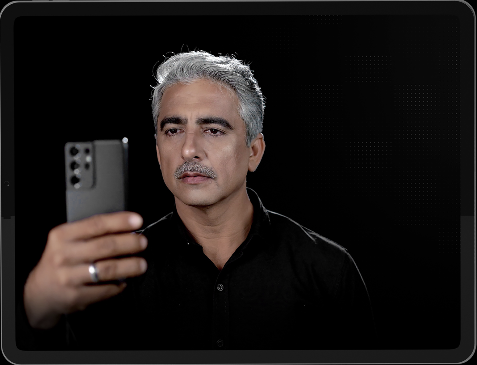
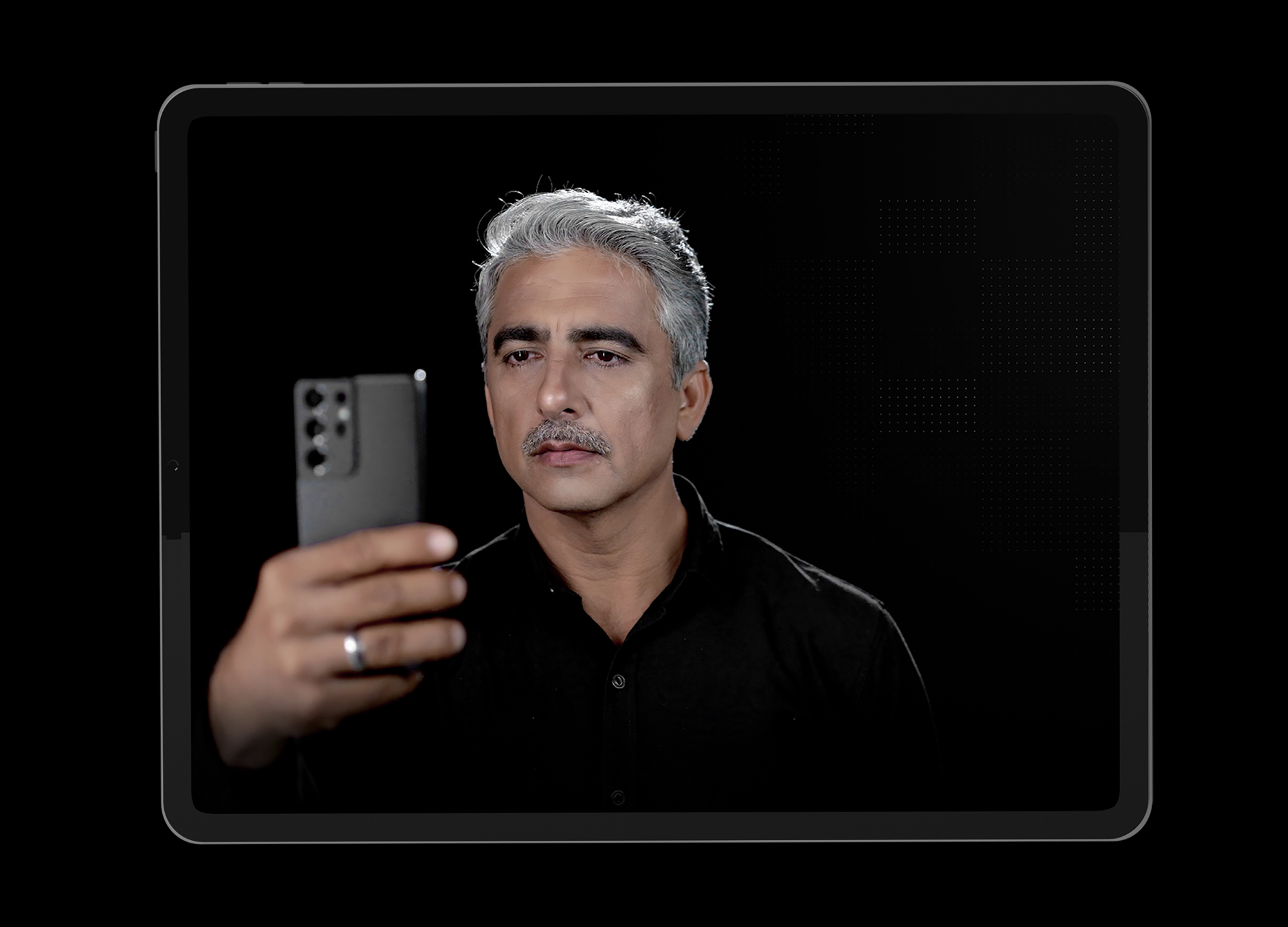
  • Video-based and contact-less
  • Runs on any device with a camera (smartphone, tablet, laptop, browser)
  • Extracts vitals within 60 seconds
  • Software-only solution, no medical hardware necessary
  • Video-based and contact-less
  • Runs on any device with a camera (smartphone, tablet, laptop, browser)
  • Extracts vitals within 60 seconds
Revolutionary Artificial Intelligence now available on Android.

Artificial Intelligence-powered SehatScan analyzes video streams using computer vision technology, signal processing, and other advanced machine learning models.

Easily share health updates with your people.

Use any social platform to effortlessly and instantly share your monitoring results with friends, families and doctors to keep them updated on your health

Our Existing rPPG patents
An Open Framework for Remote-PPG Methods and their Assessment
Giuseppe Boccignone, Donatello Conte, Vittorio Cuculo, Alessandrod’Amelio, Giuliano Grossi, Raffaella Lanzarotti

To cite this version:

Giuseppe Boccignone, Donatello Conte, Vittorio Cuculo, Alessandro d’Amelio, Giuliano Grossi, etal.. An Open Framework for Remote-PPG Methods and their Assessment. IEEE Access, 2020, 8,pp.216083-216103. ff10.1109/ACCESS.2020.3040936ff. ffhal-03046044f
HAL Id: hal-03046044
https://hal.science/hal-03046044
Submitted on 8 Dec 2020
HAL is a multi-disciplinary open accessarchive for the deposit and dissemination of scientific research documents, whether they are published or not. The documents may come fromteaching and research institutions in France orabroad, or from public or private research centers.
L’archive ouverte pluridisciplinaire HAL, estdestinée au dépôt et à la diffusion de documentsscientifiques de niveau recherche, publiés ou non,émanant des établissements d’enseignement et derecherche français ou étrangers, des laboratoirespublics ou privés

This article has been accepted for publication in a future issue of this journal, but has not been fully edited. Content may change prior to final publication. Citation information: DOI

10.1109/ACCESS.2020.3040936, IEEE Access

Date of publication xxxx 00, 0000, date of current version xxxx 00, 0000.
Digital Object Identifier10.1109/ACCESS.2017.DOI

An Open Framework for Remote-PPG Methods and their Assessment

GIUSEPPE BOCCIGNONE1 , DONATELLO CONTE2 ,VITTORIO CUCULO1 , ALESSANDRO D’AMELIO1 , GIULIANO GROSSI1 , and RAFFAELLALANZAROTTI1

1Dipartimento di Informatica - Universitàdegli Studi di Milano, Via Celoria 18, I-20133 Milano, Italy (e-mail:giuseppe.boccignone@unimi.it, vittorio.cuculo@unimi.it, alessandro.damelio@unimi.it,giuliano.grossi@unimi.it, raffaella.lanzarotti@unimi.it)
2Université de Tours, Laboratoired’Informatique Fondamentale et Appliquée de Tours (LIFAT - EA 6300)
64 Avenue Jean Portalis, 37000 Tours,France (e-mail: donatello.conte@univ-tours.fr)

Corresponding author: Giuliano Grossi(e-mail: giuliano.grossi@unimi.it).

This work has been supported by FondazioneCariplo, through the project “Stairway to elders: bridging space, time andemotions in their social environment for wellbeing”, grant no. 2018-0858.

ABSTRACT This paper presents a comprehensive framework for studying methods of pulse rate estimation relying on remote photoplethysmography (rPPG). There has been a remarkable development ofrPPG techniques in recent years, and the publication of several surveys too, yet a sound assessment of their performance has been overlooked at best, whether not undeveloped. The methodological rationale behind the framework we propose is that in order to study, develop and compare new rPPG methods in a principled and reproducible way, the following conditions should be met: i) a structured pipeline to monitor rPPG algorithms’ input, output, and main control parameters; ii) the availability and the use of multiple datasets;iii) a sound statistical assessment of methods’ performance. The proposed framework is instantiated in the form of a Python package named pyVHR (short for Python tool for Virtual Heart Rate), which is made freely available on GitHub (github.com/phuselab/pyVHR). Here, to substantiate our approach, we evaluate eight well-known rPPG methods, through extensive experiments across five public video datasets, and subsequent nonparametric statistical analysis. Surprisingly, performances achieved by the four best methods, namely POS, CHROM, PCA and SSR, are not significantly different from a statistical standpoint highlighting the importance of evaluate the different approaches with a statistical assessment.

INDEX TERMS
Remote photoplethysmography (rPPG), Python package, Statistical analysis, non-parametric statistical test, pulse rate estimation

I. INTRODUCTION
Heart beats cause capillary dilation and constriction that, in turn, modulate the transmission or reflection of visible (or infra-red) light emitted to and detected from the skin. The amount of reflected light changes according to the blood volume and these cardiac-synchronous variations can be easily captured through photoplethysmography (PPG) [1], [2], a non-invasive optoelectronic measurement technology providing the PPG signals. The latter are waveforms fluctuating according to the cardiac activity, which are also known as blood volume pulse(BVP) signal. The pulse rate variability (PRV, or heart rate variability - HRV) can then be computed from the PPG signal by measuring the time interval between two consecutive peaks of the PPG waveform.
   Recently, optoelectronic sensors based on this measurement principle have gained an important role because of

their noninvasive nature. Yet, this technique still requires contact with the skin. An advancement towards contactless technology is given by the possibility of measuring back scattered light remotely using a RGB-video camera. Such remote PPG (rPPG) measurement, formerly proposed in [3]– [5], is required in particular applications where contact has to be prevented for some reasons (e.g. surveillance, fitness, health, emotion analysis) [6]–[9]. All these works postulate that the RGB temporal traces can produce a time signal which is very close to the waveforms generated by classical PPG sensors. The traces are generally obtained by averaging the light intensity of skin at pixel level taken on some region of interest (ROI), and then concatenating them on a frame-wise basis.
    In recent years researchers have developed a number of new rPPG techniques for recovering HRV using low-cost digital

VOLUME 4, 2016
1

This work is licensed under a Creative Commons Attribution 4.0 License. For more information, see https://creativecommons.org/licenses/by/4.0/

This article has been accepted for publication in a future issue of this journal, but has not been fully edited. Content may change prior to final publication. Citation information: DOI

10.1109/ACCESS.2020.3040936, IEEE Access

Author et al.: Preparation of Papers for IEEE TRANSACTIONS and JOURNALS

cameras and making strong video-image processing [5], [10]–[16]. All these achievements are widely documented in a number of review articles covering different aspects of the non-contact monitoring of cardiac signals (see [13], [17]– [21]), and some of them have even brought to commercial solutions. This compulsive development of rPPG techniques emphasizes the importance of fair comparison of competing algorithms while promoting reproducible research. This is usually conducted on empirical basis since theoretical evaluations are almost infeasible due to the complex operations or transformations each algorithm performs. Therefore, empirical comparisons focused on publicly available benchmark datasets have become, under many respects, a cogent issue to face in establishing ranking among methods. However, existing comparisons suffer under several aspects that deserve to be thorough. These will be widely discussed in Section II, but can be broadly recapped in the following points: 1) lack of a standardized pre/post processing procedure, 2) non reproducible evaluation, 3) absence of comparison over multiple datasets, 4) unsound statistical evaluation.
   To overcome these problems and promote the development of new methods and their experimental analysis, we propose a framework supporting the main steps of the rPPG-based pulse rate recovery, together with a sound statistical assessment of methods’ performance. The framework is conceived to cope with the analysis on multiple datasets and to support each development stage of the overall Virtual Heart Rate (VHR) recovery process. This should allow researchers and practitioners to make principled choices about the best analysis tools, to fine tune process parameters or method meta-parameters, and to inquire what are the steps that mainly influence the quality of the estimations carried out.
   To concretely support experimental work within the field, the framework is instantiated into a fully open-source Python platform, namely pyVHR1 . It allows to easily handle rPPG methods and data, while simplifying the statistical assessment. Precisely, its main features lie in the following.

    Analysis-oriented. It constitutes a platform for experiment design, involving an arbitrary number of methods applied to multiple video datasets. It provides a systemic end-to-end pipeline, allowing to assess different rPPG algorithms, by easily setting parameters and meta-parameters.
    Openness. It comprises both method and dataset factory, so to easily extend the pool of elements to be evaluated with newly developed rPPG methods and any kind of video datasets.
    Robust assessment. The outcomes are arranged into structured data ready for in-depth analyses. Performance comparison is carried out based on robust non-parametric statistical tests.
    To the best of our knowledge, this proposal represents a novelty within the rPPG research field.
    In order to substantiate our framework, we analyse eight well-known rPPG methods, namely ICA [22], PCA [10],

1Freely available on GitHub: github.com/phuselab/VHR.

GREEN [5], CHROM [23], POS [13], SSR [14], LGI [15], PBV [16] (cfr. Table 1, Section III). Such methods have been selected in order to provide a substantial (although not exhaustive) set of well-known, widely adopted and methodologically representative techniques. It is worth remarking that an extensive review of all the rPPG methods proposed so far is out of the scope of the present work, whose primary concerns have been cogently remarked above.
Experiments are performed on five publicly available datasets, namely PURE [24], LGI [15], UBFC [25], MAHNOB [26] and COHFACE [27] The experimental results, some rather surprising, suggest that the four best performing methods, namely POS, CHROM, PCA and SSR, behave in the same way, leading to the conclusion that the “small” differences among these four are at chance level. The detailed results achieved by extensive tests conducted on the declared methods/datasets are reported in Section IV.
The paper is organized as follows. Section II summarizes the background and rationale about the rPPG approaches and their assessment. Section III presents the framework features and functionalities in the form of a pipeline to process the information at the various stages. Section IV reports a comprehensive statistical comparison of popular algorithms over multiple datasets using non-parametric significance hypothesis testing. Section V provides a discussion and draws some conclusions.

II. BACKGROUND AND RATIONALE
The aim of this section is to summarize the background and rationale at the base of this paper. We recall the hindrances still encountered in rPPG processing and the main challenges, currently leaving open some aspects concerning the complex nature of this remote analysis. Further, we introduce the cogent issue of statistical analysis, suitable to assess/compare methods’ effectiveness.
    As outlined in Section I, the main concerns regarding rPPG methods assessment can be summarized in the following.

1) Standardized pre/post processing.
All the considered algorithms perform some form of pre/post-processing. Such procedures heavily impact on the method’s prediction quality [20]. We believe that such procedures fall outside the method at hand, and should, therefore, be standardized in order to shed light on the quality of the rPPG extraction procedure, itself. One striking example is the face detection module; while not strictly being part of the rPPG computation from the RGB signal, it is an extremely sensible link in the chain, whose failure would lead to poor quality predictions. Other examples entail the skin detection/ROI extraction module, the filtering of the predicted rPPG signal or the spectral estimation method employed. Standardizing such procedures would allow to set up a fair comparison for all the rPPG methods involved in the analysis.

VOLUME 4, 2016
2

This work is licensed under a Creative Commons Attribution 4.0 License. For more information, see https://creativecommons.org/licenses/by/4.0/

This article has been accepted for publication in a future issue of this journal, but has not been fully edited. Content may change prior to final publication. Citation information: DOI

10.1109/ACCESS.2020.3040936, IEEE Access

Author et al.: Preparation of Papers for IEEE TRANSACTIONS and JOURNALS

2) Reproducible evaluation
A glance at the related literature reveals how there is a lack of a benchmark commonly recognised as suitable for testing rPPG methods. Indeed, experiments are generally conducted either on private datasets (e.g. [13], [14], [16],[23]), or on public ones that are not conceived for rPPG assessment (e.g. [19],[20]), preventing in both cases fair comparisons. Moreover, the different experimental conditions (e.g, illumination, subject movements, in the wild/controlled environment), or different ground truth reference signals(e.g., electrocardiogram (ECG) or BVP), are likely to prejudice comparisons, too. For instance, the public dataset Mahnob HCI-Tagging [26] was not designed for rPPG benchmarking, but rather for studying human emotions. Yet, it has been adopted to evaluate rPPG techniques [19] due to the fact that is freely available and provides recordings of the ECG signal (from which BVP can be recovered) and face videos. The same observations hold for the DEAP dataset [28] which has-been used for rPPG algorithm evaluation [20] despite being collected for the analysis of human affective states.
   Heusch and Marcel [19] proposed a novel dataset for the reproducible assessment of rPPG algorithms. In this work, authors compare three rPPG methods on the newly collected dataset (COHFACE) and on the Mahnob HCI Tagging dataset. Despite being a remarkable effort towards the principles advocated in the present research, it presents some pitfalls. Besides the absence of proper statistical evaluation, the most important is surely represented by the fact the all the analyses where carried out solely on compressed video datasets. Indeed, recent research has shown that a sound video acquisition pipeline of rPPG pulse-signal should require uncompressed coding [29]. Clearly, such recordings are often too large to be easily published online. As a consequence, many suitable datasets are often kept private. On the other hand, video compression introduces artifacts and destroys the subtle pulsatile information essential to rPPG estimation, thus making the final result inconsistent [29].

3) Comparison over multiple datasets
    A long debated issue in the pattern recognition field is represented by the bias of the dataset used when performing an analysis. As a matter of fact, running the same algorithm on different datasets may produce markedly different results. In other words, every dataset has its own bias, consequently the performances reported on a single dataset reflect such biases [30]. rPPG methods make no exception, being de facto very sensitive to different conditions [15], [24] (video compression, different lighting conditions, different setups). Hence, a sound statistical procedure for the comparison on multiple dataset is needed. To the best of our knowledge, no such analyses were proposed earlier in literature for the assessment of rPPG methods.

4) Rigorous statistical evaluation
   Typically, the performance assessment mostly relies on basic statistical and common-sense techniques, such as roughly

rank a new method with respect to the state-of-the-art. These crude methods of analysis often make the assessment unfair and statistically unsound, showing at the same time that there is no established procedure for comparing multi classifiers over multiple datasets. Here we claim that a good research practice in the field should not limit to barely report performance numbers. A partial remedy for this manifold situation probably lies in a correct experimental analysis. Many works set the focus on establishing the “winner” of a given dataset competition; as a consequence, the very question of whether the improvement over other methods is statistically significant is by and large neglected.
There is a growing quest for statistical procedures suitable for principled analyses through multiple comparisons. For instance, in domains, such as machine learning, computer vision and computational biology non parametric statistical analysis based on Friedman test (FT) has been advocated [30]–[33]. The rationale behind the FT is the analysis of variance by ranks, i.e., when rank scores are obtained by ordering numerical or ordinal outcomes. FT is well suited in the absence of strong assumptions on the distributions characterising the data. A common situation in which the FT is applied is in repeated measures design, where each experimental unit constitutes a “block” that serves in all “treatment” conditions [34]. Notable examples are provided by experiments in which k different algorithms (e.g., classifiers) are compared on multiple datasets [31]. When the FT rejects the null hypothesis because the rank sums are different, generally multiple comparisons are carried out to establish which are the significant differences among algorithms. The latter comprises the Nemenyi post-hoc test [35]. This allows for determining whether the performance of two algorithms is significantly different when the corresponding average of rankings is at least as great as its critical difference.
Of interest for the work presented here, the Nemenyi test takes into account and properly control the multiplicity effect while doing multiple comparisons [31]. It assumes that the value of the significance level α is adjusted in a single step by dividing it merely by the number of comparisons performed. In view of all these considerations, in Section IV we show how to perform the statistical comparison of rPPG algorithms under the proposed framework. Multiple datasets will be considered and the results will be ranked according to non parametric hypothesis testing.

III. THE FRAMEWORK
The functional architecture of the pyVHR framework is depicted in Figure 1. The diagram shows an end-to-end pipeline with at the heart rPPG-based pulse rate estimation algorithms. Specifically, pyVHR computes the beats per minute (BPM) estimate hˆ(t) starting with a pulse-signal in RGBspace extracted from a video sequence. We assume that the procedure takes as input a sequence of T frames and uses partially overlapped sliding windows to estimate a BVP like pulse-signal as a prelude to the final computation of hˆ(t). The overall process consists of six steps. They are schematically

VOLUME 4, 2016
3

This work is licensed under a Creative Commons Attribution 4.0 License. For more information, see https://creativecommons.org/licenses/by/4.0/

This article has been accepted for publication in a future issue of this journal, but has not been fully edited. Content may change prior to final publication. Citation information: DOI

10.1109/ACCESS.2020.3040936, IEEE Access

Author et al.: Preparation of Papers for IEEE TRANSACTIONS and JOURNALS

FIGURE 1: Overall pyVHR framework schema.

 shown in Figure 1 and briefly summarized here.

  1. Face Extraction. Given an input video v(t), a face detection algorithm computes a sequence b(t) of cropped face images, one for each frame t = 1, 2, . . . , T.
  2. ROI processing. For every cropped face, a ROI is selected, as a set of pixels containing PPG-related information, i.e. the signal q(t).
  3. RGB computation. The ROI, is used to compute the average (or median) colour intensities, thus providing the multi-channel RGB signal s(t).
  4. Pre-processing. The raw signal s(t) undergoes either detrending, frequency selective-filtering or standard normalization; the outcome signal x(t) is the input to any subsequent rPPG method.
  5. Method. The rPPG method at hand is applied to the windowed signal x(t)w(t−kτfps) (for a fixed τ ) producing a pulse signal y(t), with t = τ, 2τ, . . . , kτ, . . . ; here, fps denotes the frame rate and w the rectangular window has arbitrary size M. The number of frames used by the method to estimate the BPM for a given instant t = kτ is in the order of M = Wsfps, with Ws (sec) a time normally not exceeding 10 seconds.
  1. BVP spectrum. The BPM estimate hˆ(t) is obtained from the spectral analysis of the BVP signal y(t), either by power spectral density (PSD) or by short-time Fourier transform (STFT).

    The final stage proceeds with the error prediction analysis and the statistical assessment. The latter is normally extended to multiple methods across several datasets. Error computation is essentially based on standard metrics (for details

cfr. Section IV-B) such as Mean Absolute Error (MAE), Root-Mean-Square Error (RMSE), or Pearson Correlation Coefficient (PCC), and aims at comparing the ground truth BPM h(t) with the estimate hˆ(t) obtained via the above pipeline.
    Some of the most important processing stages, involving relevant choices within the framework, are further detailed in the following subsections.

A. FACE EXTRACTION
Given a video sequence v(t), the process starts by extracting the portion of the image corresponding to the face from each frame. The face detectors included in the framework are: dlib [36], mtcnn [37], and Kalman filter for face tracking [38]. Thus,

The signal b(t) has dimensions w×h×3×Ws, where w and h are the width and the height of the bounding box containing the face, respectively. Signal b(t) has 3 channels being coded in the RGB-color space, and depth Ws according to the time window considered.
    We include dlib mainly because it is one of the simplest and used detector in the field. However, since it often fails, especially when faces present spatial or appearance distortions, more effective face detectors are also taken into account. With the advent of deep learning, many algorithms have been developed to tackle the problem of face detection. Among them, we include mtcnn [37] that has proven its effectiveness. The drawback of this method is the time processing that prevents its adoption under real time constraints. For this reason, we also consider a simple tracking-based algorithm:

VOLUME 4, 2016
4

This work is licensed under a Creative Commons Attribution 4.0 License. For more information, see https://creativecommons.org/licenses/by/4.0/

This article has been accepted for publication in a future issue of this journal, but has not been fully edited. Content may change prior to final publication. Citation information: DOI

10.1109/ACCESS.2020.3040936, IEEE Access

Author et al.: Preparation of Papers for IEEE TRANSACTIONS and JOURNALS

face is detected on the first frame of the sequence, then Kalman filter tracking is exploited to update the coordinates of the face bounding box in subsequent frames

B. ROI PROCESSING

The aim of the ROI processing is to collect pixels contain ing the most informative signal components for heart rate estimation. Typically, best regions to extract PPG-related information encompass the entire face or are predetermined rectangular patches including, for instances, forehead, nose or cheeks. ROI selection is a critical process often requiring refinements in order to remove noise and artifacts, while preserving reliable elements for beat detection [10], [22].
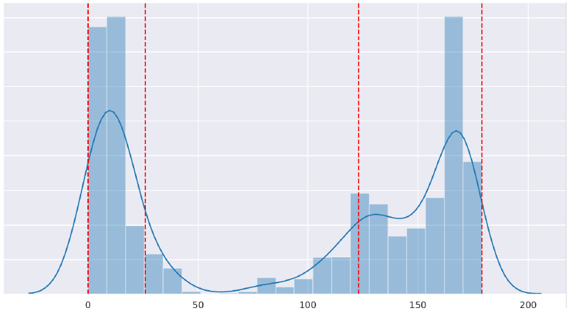
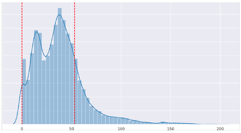
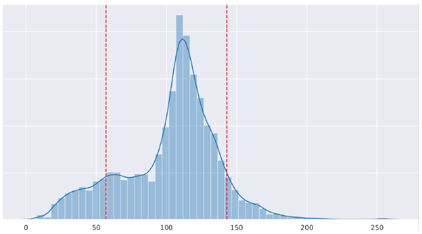
  In the pyVHR framework, we implement both rectangular ROIs and a skin detection module. As to the latter, we use simple thresholding on HSV color space (see [39]), providing two options for thresholds: fixed user-defined values, or adapted threshold calculated according to color statistics of the video frame at hand. Specifically, the face cropped image of the i-th video frame is transformed in the HSV space and empirical distributions are computed for each color channel. Thresholds are then defined as the Highest Density Interval (HDI) of the empirical distributions. HDIs represent a convenient way for summarizing distributions exhibiting skewed and multi modal shapes, for which standard dispersion metrics (standard deviations, inter quartile range, etc.) fail to provide an adequate description. HDI specifies an interval that spans most of the distribution, say 95% of it, such that every point inside the interval has higher probability than any point outside the interval [40]. Formally, given the color channel c ∈ {H, S, V }, call xc ∈ (0, 255) the possible values of the c-th color channel; the 100(1 − α)% HDI includes all those values of xc for which the density is at least as big as some value ρ, such that the integral over all those xc values is 100(1 − α)%. Namely, the values of xc in the 100(1 − α)% HDI are those such that P(xc) > ρ, where ρ satisfies R xc:p(xc)>ρ p(xc)dxc = (1 − α). In our experiments we found that a suitable value of α is α = 0.2.
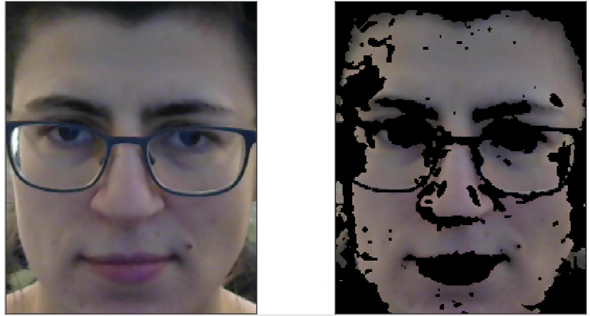
   The rationale behind this thresholding method is simple: it is assumed that in a face crop, the majority of pixel values will belong to skin; hence, thresholds should cut off all such less common pixels describing non skin areas (beards, hairs, eyes, small portions of background, etc.). Nonetheless, each face has its own features in terms of skin pigmentation, thus thresholds should exhibit an adaptive behaviour. In Figure 2, the empirical distributions of HSV values are shown; red dotted lines represent the thresholds found via HDIs. Even tually only pixels whose values lie between the thresholds are retained. Note how multiple thresholds are found when multiple modes are present. Figure 2d displays a result of skin detection; notably, non skin pixels (glasses, hair, background) are effectively removed.
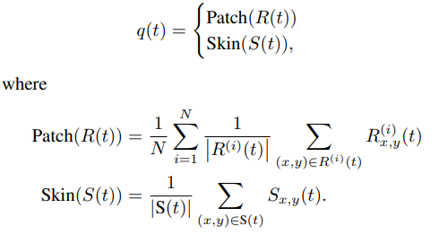
    For each frame t = 1, . . . , T, given the ROIs, either rectangular patch-based R(t) or skin-based S(t), we average over all the selected pixels to compute the output q(t) of this step. More formally, if N denotes the number of rectangular

(a) Hue
(a) Hue
(a) Hue
(a) Hue

FIGURE 2: (a), (b), (c) HSV color space thresholding viacomputation of HDIs, represented in the image by dotted redlines. (d) Original and masked face after thresholding.

patches, R(i)(t) the number of pixels in the i-th patch, and |S(t)| the number of detected skin pixels within the face, we have

C. SIGNAL PREPROCESSING
   Before computing the final photoplethysmography signal leading to the BPM estimate, a preprocessing step is applied to the raw RGB signal extracted from ROIs in order to sup press unnecessary noise and artifacts, while keeping relevant information from signal.
   A first very common preprocessing operation is band pass filtering suppressing frequency components outside the heart rate bandwidth (ranging from 40 to 220 BPM). In the framework, several band-pass filtering are provided:

  • FIR filter using Hamming window which is very effective for high frequency noise [41].
  • Butterworth IIR filter which enhances the performance of peak detection providing a better HRV estimate [42].
  • Moving Average (MA) filtering that, besides removing the high frequencies of the signal, removes various base wandering noises and motion artifacts of PPG signals, caused for example by user motion [43].

  Another kind of signal preprocessing frequently applied, and thus included in the framework, is detrending. It has-been demonstrated ([44]) that, in frequency domain, the low frequency trend components increase the power of the very low frequency (VLF) one. Thus, when using autoregressive

VOLUME 4, 2016
5

This work is licensed under a Creative Commons Attribution 4.0 License. For more information, see https://creativecommons.org/licenses/by/4.0/

This article has been accepted for publication in a future issue of this journal, but has not been fully edited. Content may change prior to final publication. Citation information: DOI

10.1109/ACCESS.2020.3040936, IEEE Access

Author et al.: Preparation of Papers for IEEE TRANSACTIONS and JOURNALS

models in spectrum estimation (like in our framework), de trending is especially recommended, since the strong VLF component distorts other components, especially the LF component, of the spectrum. The implemented detrending method [44] can be used for computing respiratory sinus arrhythmia (RSA) which component can be separated from other frequency components of HRV by properly adjusting the smoothing parameter of the method.

D. RPPG METHODS
In order to make the rPPG methods compliant with our framework, we introduced minor algorithmic changes not affecting the nature of the methods. Indeed, the ultimate goal of this work is to inquire the algorithmic principles that have inspired innovative techniques, rather than the best variants proposed for each specific method over the years. The pool of algorithms employed to carry out the experiments are listed in Table 1. They have been chosen among the most representative and widely used in this domain.
From a notational standpoint, henceforth we denote x(t) = (xr(t), xg(t), xb(t))T the preprocessed temporal trace in RGB space, resulting from the filtering-based RGB prepro cessing stage having the raw RGB signal s(t) as input. As explained at the beginning of this section, x(t) is split into overlapped subsequences, each representing samples of a finite-length multivariate measurement with t = 1, 2, . . . , M, where M = Wsfps is the number of frames selected by the sliding window defined in (1). Thus, for homogeneity, each method receives as input a chunk of the sequence x(t) and produces as output a monovariate temporal sequence y(t), a real BVP estimate coming from the application of the rPPG model.

1) ICA Method
The Independent Component Analysis (ICA) is a statistical technique aiming at decomposing a linear mixture of sources under the assumption of independence and non-Gaussianity [45]. Considering the RGB temporal traces x(t) as multivari ate measurements, the instantaneous mixture process can be expressed by

where A3×3 is a memoryless mixture matrixof the latent sources z(t) = (z1(t), z2(t), z3(t))T . The problem of sourcerecovery can be recasted into the problem of estimating the demixture matrix W≈ A−1 such that

    Problem (3) can be conceived as a problem of blind identification or separation, and many popular approaches solve it exploiting higher-order cumulants (such as kurtosis) or negentropy to measure non-Gaussianity of the mixture array (see for instance [46], [47]). Despite of the effectiveness of the method, there are nevertheless severe limitations in its applicability known as indeterminacies affecting the solutions found. Indeed, the sources are not uniquely recovered but

TABLE 1: rPPG algorithms employed to carryout the experiments and comparisons.

Method Characterization
ICA Decomposition based on blind source separation (BSS) to achieve independent components from temporal RGB mixtures.
PCA Statistical technique for extracting a subset of uncorrelated components from temporal RGB traces.
GREEN Green channel extraction preferred to red and blue because it contains less artefacts.
CHROME Chrominance-based method carrying out color channel normalization to overcome distortions.
POS It leverages on a plane orthogonal to the skin-tone in the temporally normalized RGB space.
SSR Based on spatial subspace of skin-pixels and temporal rotation measurements for pulse extraction.
LGI It provides features invariant to action and motion based on differentiable local transformations.
PBV It uses the signature of blood volume changes in different wavelengths to explicitly distinguish the pulse-induced color changes from motion noise in RGB measurements.

they are reconstructed unless arbitrary scaling, permutation and delay. Notwithstanding these ambiguities, the demixture generally preserves the waveform of the original sources retaining the most relevant time-frequency patterns particularly important in rPPG domain. Unfortunately, in order to carry out the final BPM estimation this property does not provide an answer about which component has the strongest BVP waveform among all the three. To overcome this difficulty, many solutions have been proposed in literature, but in the spirit of principled assessment motivating this framework, we implemented one of the simplest approach. It consists in calculating the normalized PSD of each source and to choose the source signal with the greatest frequency peak or signal-to-noise-ratio (SNR) within the range 40 - 220 BPM. This is quite similar to the method used in [22]. We include both JADE [46] and FastICA [47] iterative implementations of ICA in the framework since they are the most effective and stable. To determine the final source

VOLUME 4, 2016
6

This work is licensed under a Creative Commons Attribution 4.0 License. For more information, see https://creativecommons.org/licenses/by/4.0/

This article has been accepted for publication in a future issue of this journal, but has not been fully edited. Content may change prior to final publication. Citation information: DOI

10.1109/ACCESS.2020.3040936, IEEE Access

Author et al.: Preparation of Papers for IEEE TRANSACTIONS and JOURNALS

among all three candidates, we compute the PSDs S(ˆzk) with k ∈ {1, 2, 3} and set

where SNR is defined in Section III-E.

2) PCA Method
The Principal Component Analysis (PCA) is a technique broadly used in multivariate statistics and in machine learning aiming at maximizing the variances, minimizing the covariances and reducing the data dimensionality. Assuming that the multi-channel temporal trace x(t) be a realization of the random vector Z, PCA looks for an orthogonal linear transformation W ∈ R 3×3 that transforms Z to a new coordinate system Y = W Z such that the greatest possible variance lies on the first coordinate, called the first principal component. In general, if Z has finite mean E[Z] = µ and finite covariance E[(Z − µ)(Z − µ) T ] = Σ, the transformation W satisfies WT ΣW = Λ = diag(λ1, λ2, λ3), where Λ is diagonal and the i-th component of Y is called i-th principal component. Let µˆ denote the sample mean, Σˆ the sample covariance, and Wˆ the eigenvector matrix of Σˆ. Then, the sample PCA transformation can be written

In [10] PCA is mentioned for the first time in the context of pulse rate measurement, and compared against ICA, both be ing general procedures for blind source separation. However the authors do not make an explicit choice concerning the component to select for BVP approximation. In this regard, we adopt the same choices as in ICA, where frequency peaks are detected via SNR, i.e.,

3) Green Method In many works it has been reported that the green channel provides the strongest plethysmographic signal, corresponding to an absorption peak by oxyhaemoglobin ( [5], [11]). Thus, it has been argued that one of the simplest approach in estimating pulse rate via rPPG consists in 1) identifying suitable ROIs within the subject’s face, 2) calculating the average colour intensity for the green channel and, 3) by spatial averaging over the ROI, extracting the spectral content to look for highest frequency component. Thus, given the RGB temporal traces x(t), the green method boils down to consider the homonymous channel, i.e.

4) CHROM Method The CHROM method [23] has been proposed to deal with a weakness of other rPPG methods: the unpredictable normalization errors resulting from specular reflections at the

skin surface, absent in contact PPG. Briefly, light reflected from the skin consists of two components, as described by the dichromatic reflection model in [23]: a diffuse reflection component, whose variations are related to the cardiac cycle, and a specular reflection component, which shows the color of the illuminant and no pulse signal. The relative contribution of specular and diffuse reflections, which together make the observed color, depends on the angles between the camera, skin, and the light source. Therefore, they vary over time with motion of the person in front of the camera, and create a weakness in rPPG algorithms where the additive specular component is not eliminated. CHROM methods eliminate the specular reflection component by using color difference, i.e., chrominance signals. Given the RGB traces x(t), the CHROM method, after a Zero Standard Deviation Normalization, projects normalized RGB values into two orthogonal chrominance vectors XCHROM and YCHROM defined as follow:

The output rPPG signal is finally calculated by

where α = σ(XCHROM(t))/σ(YCHROM(t)), and σ(·) is the standard deviation.

5) POS Method
With the same goal of the CHROM method, that is re moving specular reflections at the skin surface, the “PlaneOrthogonal-to-Skin” (POS) method [13] defines a plane orthogonal to the skin-tone in the temporally normalized RGB space.
    In details, given x(t), POS method goes through three stages. A temporal normalization step is performed before the signal projection on the plane orthogonal to skin by

Similar to CHROM, the last step is accomplished to tune an exact projection direction within the bounded region defined by the previous step, i.e

where α is the same as CHROM. The POS approach is slightly different with respect to CHROM, because in the latter the two projected signals are antiphase, while POS directly finds two projection-axes giving in-phase signals. Moreover, to improve the SNR of the signal, the input video sequence is divided into smaller temporal intervals and pulse rate is estimated from the short video intervals; the final signal is derived by overlap-adding the partial segments

VOLUME 4, 2016
7

This work is licensed under a Creative Commons Attribution 4.0 License. For more information, see https://creativecommons.org/licenses/by/4.0/

This article has been accepted for publication in a future issue of this journal, but has not been fully edited. Content may change prior to final publication. Citation information: DOI

10.1109/ACCESS.2020.3040936, IEEE Access

Author et al.: Preparation of Papers for IEEE TRANSACTIONS and JOURNALS

6) SSR Method The rationale behind the SSR algorithm [14] is to overcome two well-known issues in existing algorithms that require skin-tone or pulse-related priors. The method consists of two steps: the construction of a subspace of skin-pixels, and the computation of the rotation angle of the computed subspace between subsequent frames. The subspace of skin-pixels is represented by the eigenvectors of an eigenvalue decomposition of the RGB space representing skin pixels.
    In detail, the vectorized matrix of skin-pixels in a video frame from RGB channels is formed, i.e. a matrix X whose dimensions are N×3, where N is the number of pixels. Then, the 3 × 3 symmetric correlation matrix C with non-negative values is computed,

Note that C is different from a covariance matrix in which the mean of X is subtracted. C is subsequently expressed in terms of the eigenvalues Λ = diag(λ1, λ2, λ3) and eigenvectors U, and matrix U is taken as a new axis system for skin-pixels.
  The model then foresees instantaneous rotation between eigenvectors (direction change) and a change of eigenvalues (energy change). To such end, a temporal stride with length l is considered and by denoting the first frame of a stride with Uτ as the reference rotation, the rotation for each t < l is given by V = Ut · Uτ . Actually, only the rotation between

In addition to the subspace rotation, by the decomposition of C, a scale/energy change of the subspace is given by

    Combining rotation and scaling, in order to obtain the time-consistent E V over multiple strides, we have to backproject it into the original RGB space:

     Finally, in a single stride, multiple E V 0 between the reference frame and succeeding frames are estimated and concatenated into a 3-dimensional trace E V . Similar to CHROM a pulse signal is derived by combining only the antiphase traces EV1 and EV2 as

and a long-term pulse-signal is estimated from subsequent strides by using overlap-adding as P¯(t−l) = P¯(t−l) − (¯p − µ(¯p)), where µ denotes the averaging operator, eventually providing the output

7) LGI Method Local Group Invariance method [15] aims at finding a new feature space from preprocessed signal x(t), in which rPPG is more robust to nuisance factors, like human movements and lightness variations. The projection into this new space is very similar to that of the SSR method and it is based on matrices C in Eq. (5) and U introduced above. A projection operator O onto this new space is calculated by

where I is the identity matrix.
    Finally, the rPPG signal is computed by projecting the input signal x(t) with matrix O is given by

8) PBV Method
In [16] the authors show that the optical absorption changes caused by blood volume variations in the skin occur along a very specific vector in the normalized color channel space and this is called Pulse Blood Volume (PBV) vector. It is calculated as

    where X = {Xr, Xg, Xb} is the matrix representation of the pre-processed signal x(t) for the considered window, and σ(·) is the standard deviation operator.
     The output signal is finally computed by the projection

where M is the orthogonal matrix

and k is a normalization factor.

E. SPECTRAL ANALYSIS
To assess the pulse rate variability (PRV), spectral methods are commonly used. The time-domain approaches based on interbeat interval (IBI) provided by ECG traces are more accurate, but they are rarely used due to the difficulty in estimating RR-peaks in time series [48]. For this reason, methods relying on pulse-wave analysis are more commonly used, being considered more effective and stable for the estimation of heart rate variability [12]. This fact is witnessed by a number of publications reporting universally good agreement between PRV and HRV, even if this concordance may be susceptible of many variables such as experimental conditions and postures (see [48] and the citations thereof).
   To face a stochastic scenario like that offered by rPPG measurements, two relevant issues should be taken into account: the basic periodicity of the underlying phenomenon and the random effects introduced by noise. Based on these assumptions, almost all methods used to capture the peaked patterns within the rPPG waveforms consider more reliable the frequency domain than the temporal one. A further reason

VOLUME 4, 2016
8

This work is licensed under a Creative Commons Attribution 4.0 License. For more information, see https://creativecommons.org/licenses/by/4.0/

This article has been accepted for publication in a future issue of this journal, but has not been fully edited. Content may change prior to final publication. Citation information: DOI

10.1109/ACCESS.2020.3040936, IEEE Access

Author et al.: Preparation of Papers for IEEE TRANSACTIONS and JOURNALS

supporting this approach is that the noise spectrum has almost certainly a different spectral line, helping in discriminating the most informative frequency peaks.
    Under such circumstances, the usual spectral analysis is performed via PSD estimation, which provides information about power distribution as a function of frequency. It inherently assumes that the signal is at least weakly stationary to avoid distortion in time- and frequency-domain. In order to assure a weaker form of stationarity, here we compute the PSD on small intervals, e.g. 5÷10 seconds, so as to preserve the significant peaks in the pulse frequency-band ([40, 240] BPM). In this framework, the PSD is accomplished through the discrete time Fourier transform (DFT) using the Welch’s method, which employs both averaging and smoothing to analyze the underlying random phenomenon [49].
    Given a sequence y(t) of length N yielded by averaging ROIs on as many video frames, with t = t0 + nT and n = 0, 1, . . . , N − 1, the sequence is split into K segments of length L, with a shift of S samples between adjacent segments (resulting in an overlap of L − S points). Here T represents the time between two successive frames, i.e, T = 1/fps. By denoting with x(0), . . . , x(N − 1) the rPPG signal y(t), for each segment k (k = 0 to K −1) a windowed DFT is computed by

where t` = (k − 1)S, . . . , L + (k − 1)S − 1 and frequencies ν = κ/L, with κ ∈ Ω M= {−L/2−1, . . . , L/2}. These DFTs in turn provide the per segment periodogram

where Wp denotes the window power.
    The overall PSD is then yielded by averaging over periodograms:

Naturally, the frequency f expressed in Hz (PSD is plotted vs Hz) ranges from (−1/2T + 1/LT) and 1/2T achieved by simple conversion from the normalized frequency ν expressed in Hz-sec and ranging in Ω. After the computation of the PSD estimate Sx, the peak provided by

results in the frequency

corresponding to PSD maxima, carried out by Welch’s method.
    Clearly L is the dominant parameter and it is worth noting that in terms of frequency resolution at 60 BPM, short intervals (e.g. less than 20 sec) should entail very coarse estimates of BPMs. For the latter and previous reasons, here we increase the resolution of the DFT setting L = 2048,

which results in a final reasonable compromise for temporal video segmentation of less than 10 seconds.
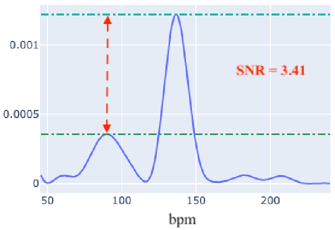
     A useful metric to compare traces is the SNR expressed in terms of frequency power spectrum. To select better PSD shapes emphasizing the fundamental frequency, a simple way is to maximize the ratio between the peak of the first harmonic and other spurious peaks appearing in the rPPG signal PSD. Figure 3 shows an example where the main lobe identifies the fundamental frequency and the maximum sidelobe the noise.

FIGURE 3: SNR: ratio between the magnitude of main lobe and the maximum magnitude of sidelobes.

     This metric is definitel y useful for ICA and PCA methods in order to identify the best trace among the three (one for each color channel) carried out by methods.

F. THE GROUND TRUTH SIGNAL
Public datasets provide ECG or BVP signals as ground truth, while methods usually provide BPM estimation on a video. It is therefore necessary to estimate HRV from ECG or BVP signals in order to compare method outcomes with ground truth. HRV measurement is not simple and this problem is well known in literature ( [50]–[52]). A variety of recording techniques have been proposed, which can roughly be categorized into time and frequency domain-based.
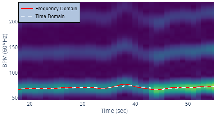
      In time domain, HRV is calculated from RR intervals occurring in a chosen time window (usually between 0.5 and 5 min). In frequency domain, HRV is computed by calculating the spectrogram of the BVP signal (by STFT computation). Both techniques present advantages and disadvantages (see [50] for an in-depth analysis). Figure 4 shows that however in general the estimate achieved by both time and frequency domain are very close, with a MAE (see Section IV-B) less than 1 BPM. So in the pyVHR framework we use only the frequency domain technique (i.e. PSD) to estimate the ground truth from ECG or BVP signal.
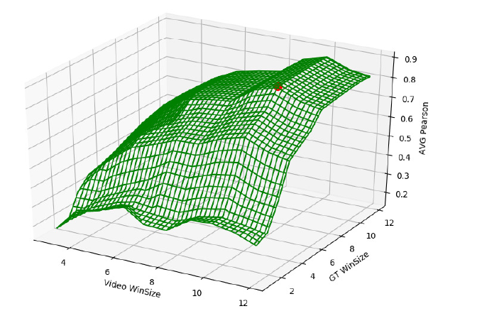
      An important aspect rising from the previous considerations is the window size setting for both video and ground truth analysis. Figure 5 displays the results of extensive simulations comparing different overlapped window sizes (Ws vs ground truth window size) for BPM estimation using POS method on the UBFC dataset. As can be noted, the

VOLUME 4, 2016
9

This work is licensed under a Creative Commons Attribution 4.0 License. For more information, see https://creativecommons.org/licenses/by/4.0/

This article has been accepted for publication in a future issue of this journal, but has not been fully edited. Content may change prior to final publication. Citation information: DOI

10.1109/ACCESS.2020.3040936, IEEE Access

Author et al.: Preparation of Papers for IEEE TRANSACTIONS and JOURNALS

FIGURE 4: The spectrogram calculated on one video of the PURE dataset. The estimated HRV by frequency analysis and by time analysis (RR peaks difference) are shown in red and (dashed) white respectively. The MAE between these two signals is 0.87 BPM.

highest PCC is obtained when setting video winSize= 10 and GT winSize = 7. For higher values no significant increase in PCC was found. Although Figure 5 provides the results obtained with the POS method, the same analysis conducted with other methods yielded similar results. Unsurprisingly, we found that (regardless to the method) wider video win Sizes produce better predictions; eventually a plateau is reached around 10 seconds. Similar considerations apply to the ground truth signal winSize, where typically the plateau is attained at around 7 seconds.
    According to this analysis, in all our experiments (see Section IV) we set the video window size equal to Ws = 10 sec and ground truth window size equal to 7 sec.

FIGURE 5: Average Pearson Correlation Coefficient (PCC) between ground truth and predicted heart rate using the POS method. PPC values are computed for different values of video winSize and ground truth (GT) winSize on the UBFC dataset. The red dot indicates the optimum.

IV. DATA AND STATISTICAL ANALYSES
In this section we report a comprehensive statistical comparison of the algorithms outlined in the previous section over multiple datasets by safe, yet robust non-parametric tests. As motivated by many works in different scientific domains, we apply the Friedman test [53] instead of standard ANOVA, because it relaxes the assumptions of normality and equality of variances of the residuals.
   Moreover, we are not only interested in knowing whether any difference exists among algorithms, but also in discovering which method is significantly different from each other (and the FT is not designed for this purpose). To this end, we apply the so-called post-hoc tests to find out which methods actually differ [31].
     In the rest of this section we describe the evaluation metrics used to assess the performance quality, and the nonparametric hypothesis testing procedure as applied to a pool of six benchmarking datasets. The provided results have been carried out either referring to tests on each dataset separately, or on tests across datasets.

A. BENCHMARK DATASETS
The framework accounts for a multi-dataset analysis. Namely, we consider data from 6 datasets, briefly described in the following.

Mahnob [26]. Although this database was mainly conceived for emotion analysis, it has been adopted for testing rPPG algorithms, [54], [55], even though it applies a strong compression on the videos. 30 participants (17 females and 13 males, aging between 19 to 40 years old) were shown fragments of movies and pictures, while monitoring them with 6 video cameras, each capturing a different view point, a head-worn microphone, an eye gaze tracker, as well as physiological sensors measuring ECG, electroencephalogram, respiration amplitude, and skin temperature. Since ECG data is available, this dataset has been widely used also for heart rate estimation, after processing ECG data to create heart rate ground truth. Mahnob dataset contains videos compressed in H.264/MPEG-4 AVC compression, bit rate ≈ 4200kb/s, 61 fps, 780 × 580 pixels, which gets ≈ 1.5 × 10 − 4 bits per pixel, resulting in an heavy compression. In this paper only a subset of the video data has been used.

Cohface [27]. This dataset contains 160 one-minute-long RGB video sequences, synchronized with the heart-rates and breathing-rates of the 40 subjects (12 females and 28 males) recorded. Each participant was asked to sit still in front of a webcam to allow capturing the whole face area. Two types of lighting conditions were considered: studio, using a spot light, and natural light. The videos are compressed in MPEG-4 Visual, i.e. MPEG-4 Part 2, bit rate ≈ 250kb/s, resolution 640 × 480 pixels, 20 frames per second, which gets ≈ 5×10−5 bits per pixel. In other words, the videos were heavily compressed.

PURE [24]. This database comprises 10 subjects (8 male, 2 female) that were recorded in 6 different setups resulting

VOLUME 4, 2016
10

This work is licensed under a Creative Commons Attribution 4.0 License. For more information, see https://creativecommons.org/licenses/by/4.0/

This article has been accepted for publication in a future issue of this journal, but has not been fully edited. Content may change prior to final publication. Citation information: DOI

10.1109/ACCESS.2020.3040936, IEEE Access

Author et al.: Preparation of Papers for IEEE TRANSACTIONS and JOURNALS

in a total number of 60 sequences of 1 minute each. Lighting condition was frontal daylight, with clouds changing illumination conditions slightly over time. People were positioned in front of the camera with a distance of about 1.1 meters, capturing uncompressed cropped resolution images of 640 × 480 at 30Hz. Reference pulse rate was captured using a finger clip pulse oximeter with sampling rate of 60 Hz. Six different setups have been recorded: Steady (S); Talking (T); Slow translation (ST); Fast translation (FT); Small rotation (SR); Medium rotation (MR).
UBFC [25]. This dataset is composed of 50 videos, synchronized with a pulse oximeter finger clip sensor for the ground truth. Each video is about 2 min long recorded at 30Hz with a resolution of 640 × 480 in uncompressed 8- bits RGB format. The authors divided this dataset into two subsets: the first one, UBFC1 is composed by 8 videos, in which participants were asked to sit still; the second one, UBFC2 is composed by 42 videos, in which participants were asked to play a time sensitive mathematical game that aimed at augmenting their heart rate while simultaneously emulating a normal human-computer interaction scenario. Participants were sitting frontal to a camera placed at a distance of about 1 meter.
LGI [15]. This database is designed for the heart rate estimation from uncompressed face videos acquired in the wild. It is recorded in four different sessions: 1) a resting scenario with neither head motion or illumination changes, 2) head movements are allowed (with static lighting), 3) a more ecological setup, where people are recorded while performing exercises on a bicycle ergometer in a gym; 4) urban conversations are recorded including head and facial motions as well as natural varying illumination conditions. Videos were captured at 25Hz while the pulse sampling rate was 60Hz. It’s worth remarking that although the original dataset nominally provides 25 subjects, at the time of writing only 6 are officially released and therefore used in the analysis.

   In literature, all these datasets have been adopted to test rPPG algorithms. However it has also been pointed out how the compression can destroy and pollute the subtle pulsatile information essential to rPPG. In [56] it has been claimed that uncompressed videos could increase SNR due to information being lost during the video compression process. Similarly, in [29] a more in depth analysis has been conducted, aiming at finding an acceptable level of compression, indeed necessary in real world applications.

B. EVALUATION METRICS
We use three common metrics to evaluate the performance of the methods that are briefly recalled here. Procedurally, to measure the quality of the bmp estimate hˆ(t) with respect to the ground truth h(t) with a cadence dictated by a fixed time τ , i.e., t = τ, 2τ, . . . , Nτ we split each trial (see section III) into epochs of Ws seconds with Ws − τ overlap seconds only when τ < Ws. If the video frame sequence is made by T frames, N = T /(τ fps) is the number of samples of

sequence hˆ(t), being fps the video frame rate. The following quantities were used to assess estimation performance for the epochs of each participant.

MAE. The Mean Absolute Error is calculated as:

In all experiments carried out (see next section), τ = 1 sec, which give about 60 BPM, and elapsed video time are no more than 120 seconds.
RMSE. The Root-Mean-Square Error measures the difference between quantities in terms of the square root of the average of squared differences, i.e.

RMSE represents the sample standard deviation of the absolute difference between reference and measurement, i.e., smaller RMSE suggests more accurate extraction.
PCC. Pearson Correlation Coefficient represents the correlation between the estimate hˆ(t) and the ground truth h(t):

    where µˆ and µ denote the means of the respective signals.

C. NONPARAMETRIC STATISTICAL TESTS
The a forementioned performance measures are now used to perform the statistical analysis. By following [31] each metric is analyzed via the Friedman Test (FT) followed by the associated post-hoc analysis.
    To perform the FT, we apply the repeated measures design in which k classifiers are compared on multiple datasets. The observed data is arranged in a tabular form, where the columns represent the classifiers (i.e., “groups” in standard statistical test notation) and the rows the datasets (“blocks”). Observations in different blocks are assumed to be independent, but obviously this assumption does not apply to the observations within a block.
     Denote xj,d the performance measure for the j-th method on the d-th dataset (with j = 1, . . . , k and d = 1, . . . , n). The xj,d values are sorted with respect to j so that each observation within a block receives a distinct rate among the first k integers, thus yielding the values rj,d ∈ {1, . . . , k} indicating the rank of j-th algorithm on the d-th dataset.
     A rank of rj,d tells that the method j outperformed k−rj,d methods on the dataset d. The average rank for any j over the datasets is defined as Rj = (1/n) P i rj,d. Under the null hypothesis, i.e., no difference between the algorithms, their ranks Rj should be equal, and the statistic is

VOLUME 4, 2016
11

This work is licensed under a Creative Commons Attribution 4.0 License. For more information, see https://creativecommons.org/licenses/by/4.0/

This article has been accepted for publication in a future issue of this journal, but has not been fully edited. Content may change prior to final publication. Citation information: DOI

10.1109/ACCESS.2020.3040936, IEEE Access

Author et al.: Preparation of Papers for IEEE TRANSACTIONS and JOURNALS

which follows a chi-squared distribution with k−1 degrees of freedom. The FT rejects the null-hypothesis at a pre-specified significance level α when the test statistic (8) exceeds the 100(1 − α)th percentile of the limiting chi-squared distribution of χ2/F with k − 1 degrees of freedom [53].
    When the null-hypothesis is rejected, a post-hoc test, such as Nemenyi test [35], can be performed to establish which are the significant differences among the algorithms. If the difference in average rank between two methods i and j exceeds a critical difference CDα,k,n, i.e., Ri − Rj > CDα,k,n then the performance of algorithm i is better than the performance of algorithm j with confidence α. The critical difference is given by [31]

where qα,k is drawn from the studentized range distribution and depends on both the significance level α and the number of methods compared k (see Table 5 in [31]). Put simply, the critical difference is the minimum required difference in rank sums for a pair of algorithms to differ at the prespecified level of significance α.

D. EXPLORATORY ANALYSIS OF PERFORMANCE
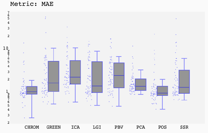
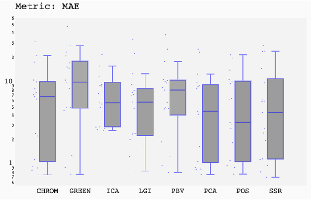
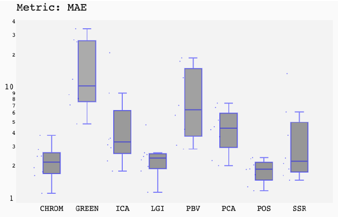
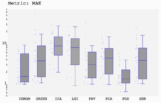
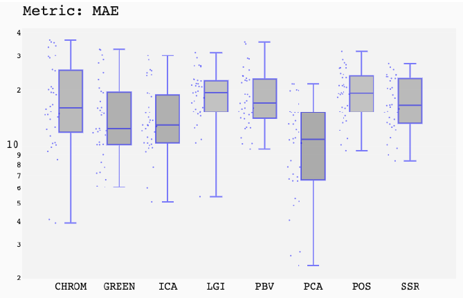
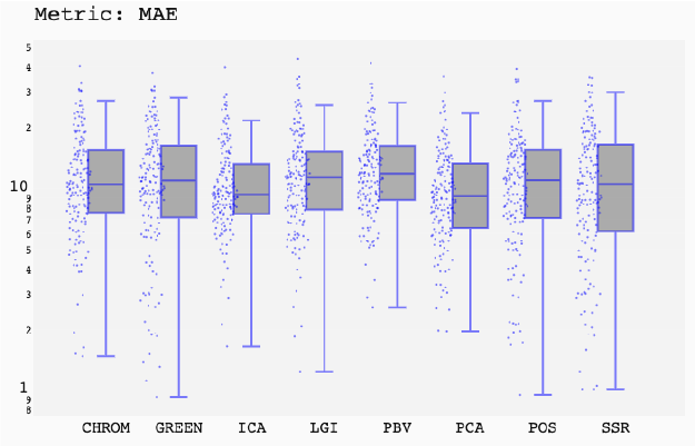
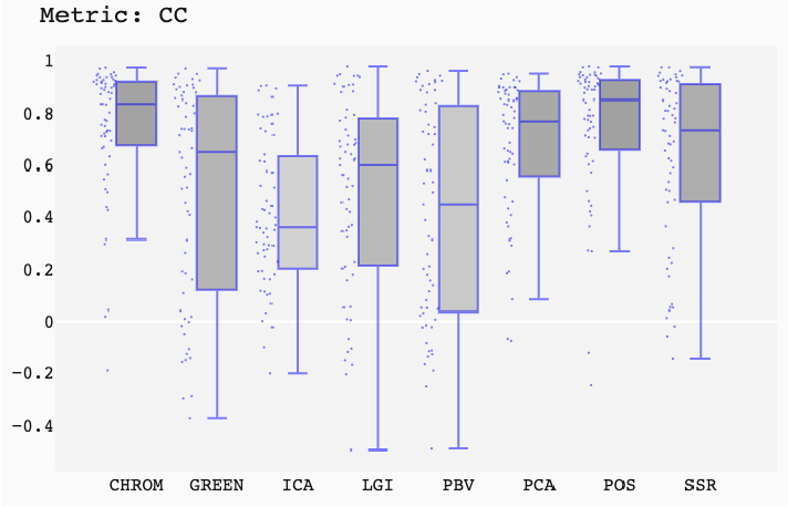
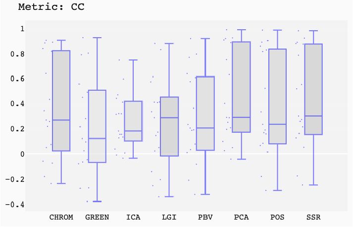
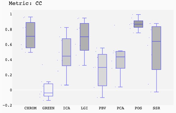
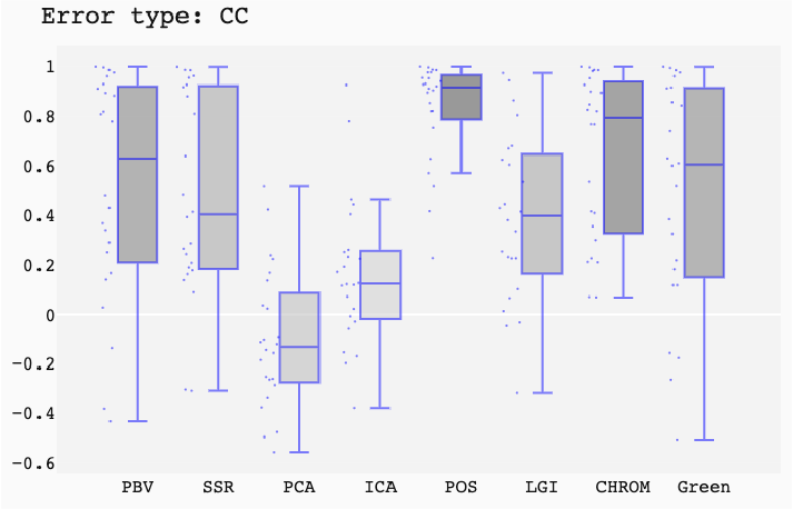
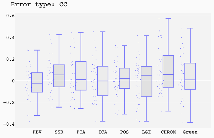
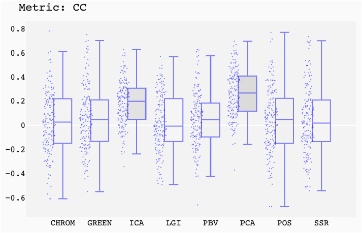
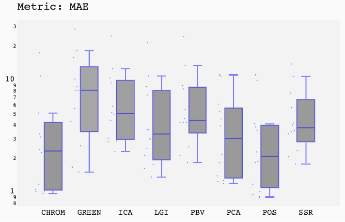
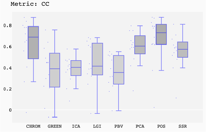
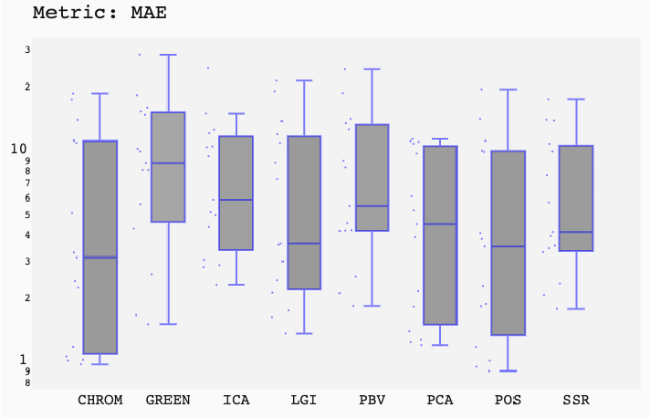
We first provide a summary, via box plots, of the overall performances achieved by the eight rPPG algorithms over the six benchmark datasets (UBFC dataset is split in two parts, namely UBFC1 and UBFC2, as described in previous section). By measuring the central tendency via the median we are able to elicit information about the underlying distribution as well as to identify possible outliers (their character, the amount, etc.). Figures 6 and 7 present the standard boxplots computed by pyVHR framework and associated to MAE and PCC metrics, respectively. Data are plotted in log scale in order to emphasize the best values for each metric; the boxes are put in gray scale with the intensity proportional to the median value.
     The general consideration that can be drawn at a glance (besides the log-scale) is that the fences defined by the whiskers are far too small with respect to outliers, and probably asymmetry or tail heaviness is a distinctive character of all distributions. It is also evident that the extremities of upper whiskers go beyond those of the lowers in almost all cases. It’s worth to notice also that the high variability of the results does not lay down an absolute winner or loser among methods against all datasets. Instead, it is beyond doubt that methods perform consistently better on uncompressed video datasets (PURE, LGI and UBFC) whereas it is quite impossible to establish a sound ranking of the methods for compressed video datasets (MAHNOB and CHOFACE). Besides the median, also the interquartile range, IQR, (defined as the difference between the third and first quartile and representing the box size), covering the central 50% of the data, provides useful insights for the assessment procedure. By inspecting the IQRs depicted in the figures, it is worth noticing that in general the methods POS and CHROM

provide better median MAE and PCC values, albeit showing less spread with respect to the others.
    A more rigorous and statistically sound assessment of the difference in medians between methods is left to the forthcoming analysis through the Friedman test.

E. INFERENTIAL ANALYSIS OF PERFORMANCE

1) Single Dataset Analysis

In all experiments in the single dataset condition, the FT, whose statistics is defined in (8), rejected the null hypothesis with very low p-values (p < 10−3 ). To establish the significant differences between the algorithms post-hoc analysis has been performed via Nemenyi test, Critical values (Eq. (9)) were computed followed by pairwise comparisons. These are reported, for each dataset, in Table 2.

TABLE 2: Nemenyi test critical values CDα,k,n for comparing the 8 rPPG methods among n (size of each dataset) videos at the α = 0.95 confidence level.

Dataset Size (n) CD
PURE 59 1.36
LGI 17 2.54
UBFC1 8 3.71
UBFC2 24 2.14
MAHNOB 36 1.74
COHFACE 164 0.81

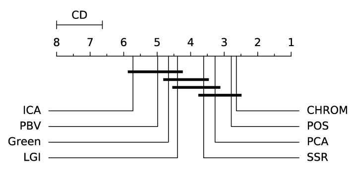
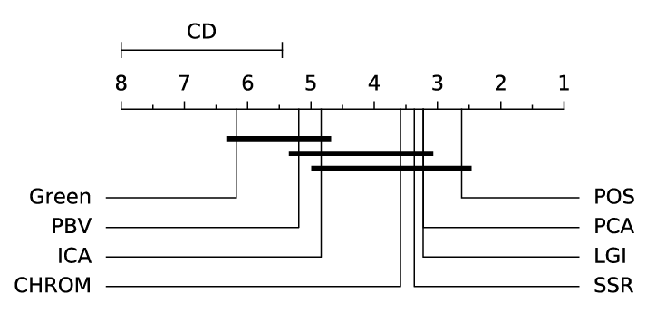
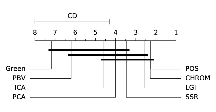
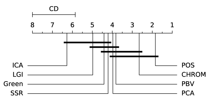
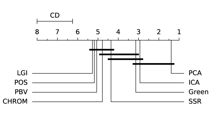
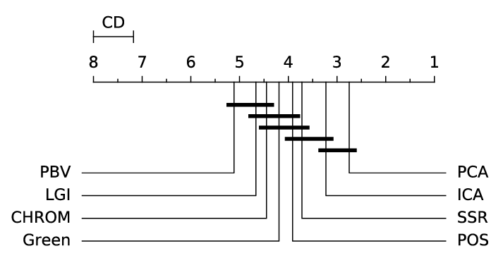
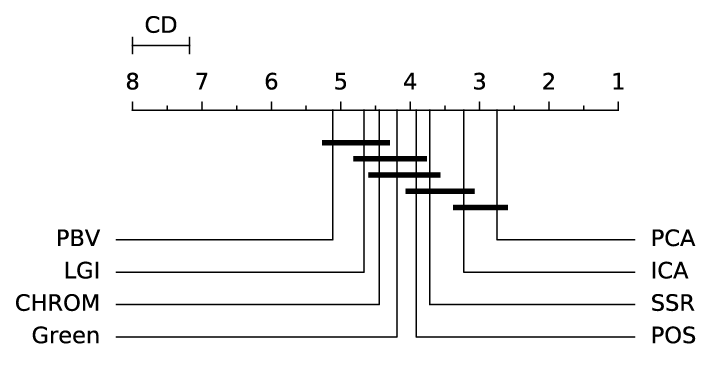
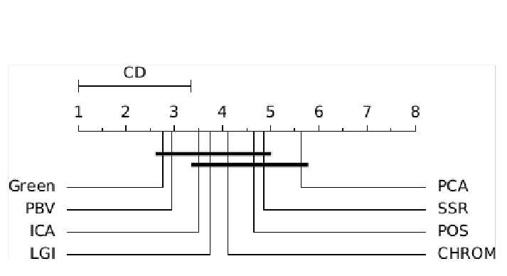
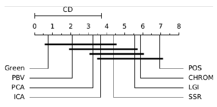
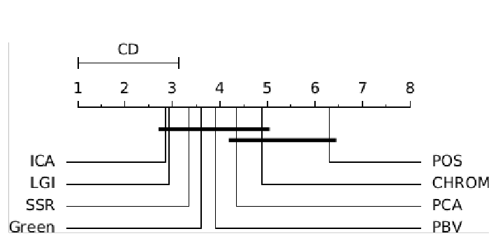
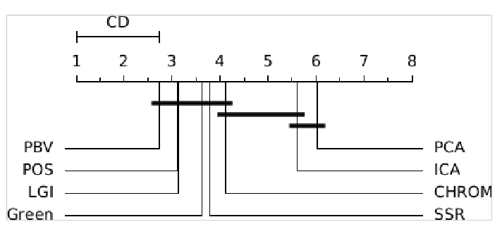
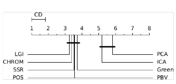
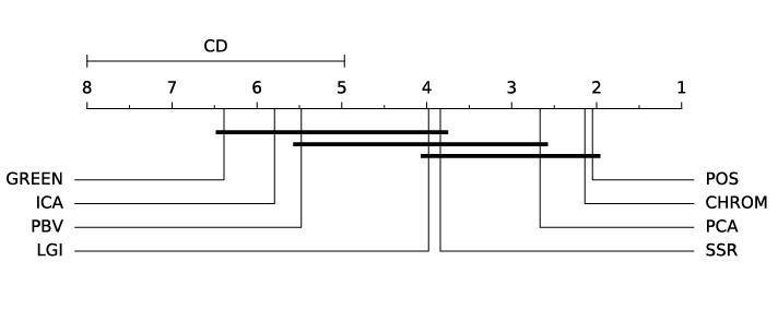
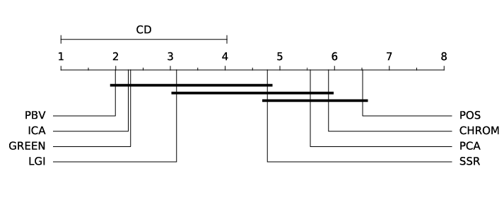
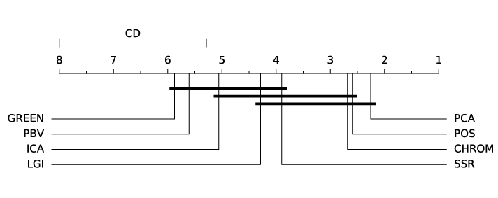
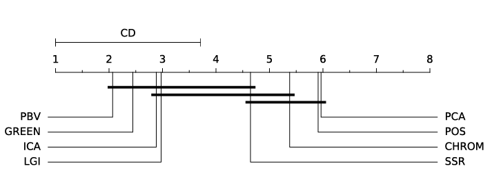
    As suggested in [31], differences arising from post-hoc tests can be visually represented with simple diagrams connecting groups of methods that are not significantly different. Figures 8 and 9 display the critical differences through the so-called critical differences diagram (CD), a succinct way to display the differences in methods’ performance.
    The top line in the diagram is the axis where the average ranks of methods are plotted. The axis is turned so that best performing methods are displayed to the right. Note that depending on the metric adopted, either MAE or PCC, the best ranking method can be the one with the lowest or highest rank respectively. The figures display the CD diagrams obtained from the FT followed by the post-hoc Nemenyi test with a significance level of 95%. A line connecting two or more methods indicates that there are no statistical differences between them. The CDs are also shown above the graph.
    CDs show a wide ranking variety depending on dataset and metric used. The groups of rPPG methods that behave the same change accordingly, providing a clear picture of the impossibility to establish an absolute pool of winners across datasets. The investigation also give evidence of the usefulness and strength of multiple comparison statistical procedures to analyse and select the best methods for a single dataset.

VOLUME 4, 2016
12

This work is licensed under a Creative Commons Attribution 4.0 License. For more information, see https://creativecommons.org/licenses/by/4.0/

This article has been accepted for publication in a future issue of this journal, but has not been fully edited. Content may change prior to final publication. Citation information: DOI

10.1109/ACCESS.2020.3040936, IEEE Access

Author et al.: Preparation of Papers for IEEE TRANSACTIONS and JOURNALS

(a) PURE.
(b) LGI.
(c) UBFC1.
(d) UBFC2.
(e) MAHNOB.
(f) COHFACE.

FIGURE 6: Mean Absolute Error (MAE) for each dataset and each rPPG method represented by the box and whisker plot (in log-scale). The median is indicated by the horizontal blue line, the first and third quartile are indicated by the blue box, and the whiskers extend to the most extreme data points not considered outliers.

VOLUME 4, 2016
13

This work is licensed under a Creative Commons Attribution 4.0 License. For more information, see https://creativecommons.org/licenses/by/4.0/

This article has been accepted for publication in a future issue of this journal, but has not been fully edited. Content may change prior to final publication. Citation information: DOI

10.1109/ACCESS.2020.3040936, IEEE Access

Author et al.: Preparation of Papers for IEEE TRANSACTIONS and JOURNALS

(a) PURE.
(b) LGI.
(c) UBFC1.
(d) UBFC2.
(e) MAHNOB.
(f) COHFACE.

FIGURE 7: Pearson’s correlation coefficients (PCC) for each dataset and each rPPG method represented by the box and whisker plot. The median is indicated by the horizontal blue line, the first and third quartile are indicated by the blue box, and the whiskers extend to the most extreme data points not considered outliers.

VOLUME 4, 2016
14

This work is licensed under a Creative Commons Attribution 4.0 License. For more information, see https://creativecommons.org/licenses/by/4.0/

This article has been accepted for publication in a future issue of this journal, but has not been fully edited. Content may change prior to final publication. Citation information: DOI

10.1109/ACCESS.2020.3040936, IEEE Access

Author et al.: Preparation of Papers for IEEE TRANSACTIONS and JOURNALS

(a) PURE.
(b) LGI.
(c) UBFC1.
(d) UBFC2.
(e) MAHNOB.
(f) COHFACE.

FIGURE 8: Critical differences diagram (CD) obtained from the Friedman test followed by the post-hoc Nemenyi test comparing the rPPG approaches under MAE metric. Groups of methods that are not significantly different (at p = 0.05) a reconnected.

VOLUME 4, 2016
15

This work is licensed under a Creative Commons Attribution 4.0 License. For more information, see https://creativecommons.org/licenses/by/4.0/

This article has been accepted for publication in a future issue of this journal, but has not been fully edited. Content may change prior to final publication. Citation information: DOI

10.1109/ACCESS.2020.3040936, IEEE Access

Author et al.: Preparation of Papers for IEEE TRANSACTIONS and JOURNALS

(a) PURE.
(b) LGI.
(c) UBFC1.
(d) UBFC2.
(e) MAHNOB.
(f) COHFACE.

FIGURE 6: Mean Absolute Error (MAE) for each dataset and each rPPG method represented by the box and whisker plot (in log-scale). The median is indicated by the horizontal blue line, the first and third quartile are indicated by the blue box, and the whiskers extend to the most extreme data points not considered outliers.

VOLUME 4, 2016
16

This work is licensed under a Creative Commons Attribution 4.0 License. For more information, see https://creativecommons.org/licenses/by/4.0/

This article has been accepted for publication in a future issue of this journal, but has not been fully edited. Content may change prior to final publication. Citation information: DOI

10.1109/ACCESS.2020.3040936, IEEE Access

Author et al.: Preparation of Papers for IEEE TRANSACTIONS and JOURNALS

2) Cross-dataset Analysis

Thorough this paper, we have considered the results obtained in a experimental study regarding 8 well-known algorithms using a benchmark suite of 5 datasets we have selected among the most representative.
    To finally highlight the significant statistical differences among the various algorithms, we further split the datasets into 15 subdatasets, as shown in Table 3. The reason is twofold: on the one hand this split reflects the peculiar differences within each dataset, also motivated by the different algorithm behaviour on each subdataset. On the other hand it allows to increase the number of blocks that, as a rule of thumb, for the FT should be greater than 10 [31]. In addition, our analysis considers a further partition between an uncompressed video collection (top 12 of the table) and a compressed video one (least 3 at the bottom). The rationale of this distinction relies on the fact that compression certainly is the feature that more than anything else affects both the performances of each rPPG approach and the results of nonparametric statistical tests.
     Table 3 also reports the MAE and PCC obtained for the 8 algorithms over the 15 datasets considered. For the compressed datasets (top of the table), the lowest median is obtained by POS method for the MAE metric (lowest IQR by CHROM) , whereas the highest PCC median values is produced by POS algorithm (the lowest IQR by others). In turn CHROM provides the best values when results are extended to all datasets (complete table), but the same does not hold for for IQR which has various winners. Boxplot of Figures 11 and 10 synthetically visualize all comparisons. As for the FT, the p-values = 9 · 10−6 computed through the χ 2 statistics, strongly suggests the existence of significant differences among the algorithms considered. Nemenyi tests results with critical values at 95% are provided in Figs, 11-(c) and 11-(d).
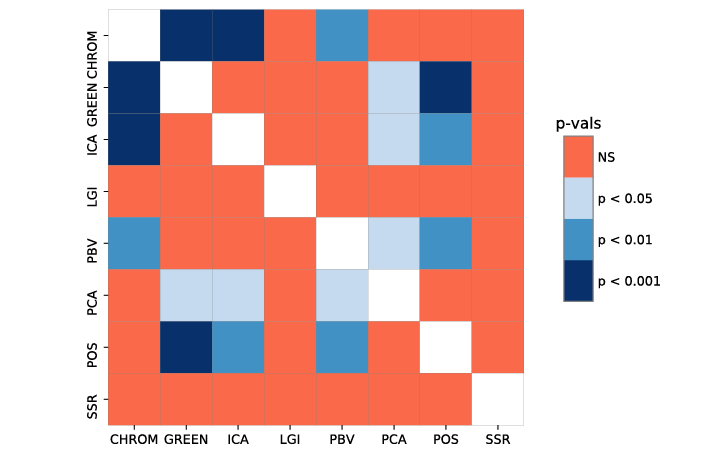
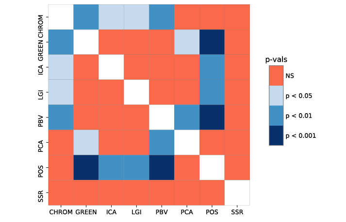
     Surprisingly, it turns that the performances achieved by the four best methods, namely POS, CHROM, PCA and SSR, are not significantly different from a statistical standpoint.
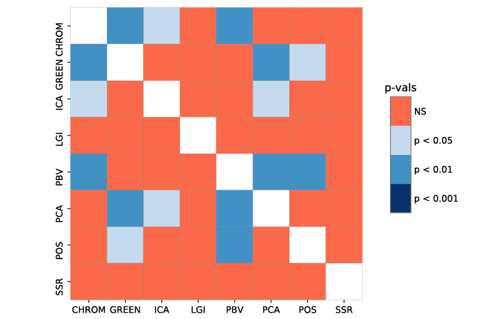
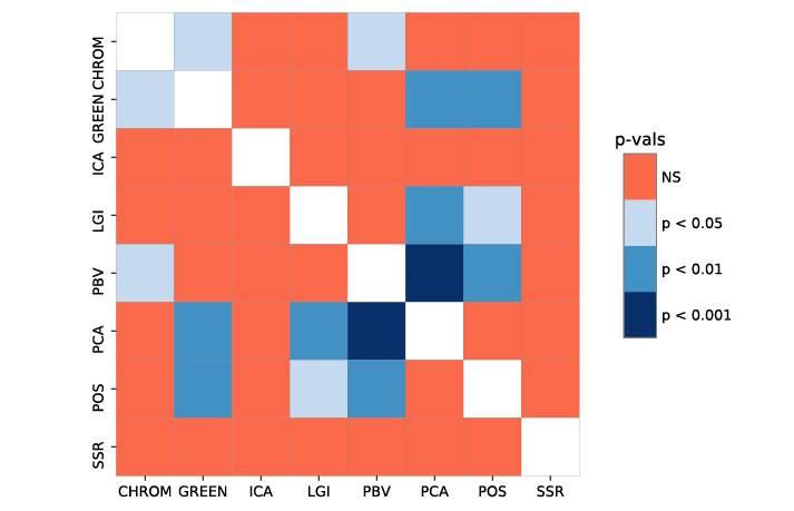
     Using a three different levels of significance, namely α ∈ {0.05, 0.01, 0.001}, Figures 10-(e) and 10-(f) display in the form of heatmaps the various hypotheses rejected/accepted by the Nemenyi method for the uncompressed video datasets. In particular, the heatmaps collect a family of 28 hypotheses (all pairs of algorithms) highlighting which algorithms achieve improvements with respect to others, at each given level of significance. The value of significance levels are marked with intensity proportional blue color; alternatively, they are marked with NS to claim that the difference is not significant. It should be noted that with 8 hypotheses for MAE and 10 for PCC, the differences between pairwise and multiple comparisons become apparent. As for the general case, including uncompressed and compressed videos, the Figures 11-(e) and 11-(f) show the results of the same statistical procedure applied to the uncompressed videos. Note that here with 8 hypotheses for MAE and 8 for PCC the differences are substantial.

     Taking a look at the second row in Figure 10-(e) and 10- (f), it can be noticed that there is a significant difference between POS and GREEN (p < 0.001) for both metrics. On the other hand, differences between CHROM and GREEN or ICA exhibit less pronounced (although still significant) differences (p < 0.05).

V. CONCLUSIONS

Pulse rate estimation using remote photoplethysmogram (rPPG) is an on-going and growing research area. In many respects it is also a mature discipline encompassing a remarkable amount of results both in terms of algorithmic principles introduced and also in relation to the acquired knowledge over time. However, besides the experience gained so far in the field, many important issues still remain in the background. We refer in particular to the careless attitude exhibited during the experimental sessions aiming at fairly comparing new proposed techniques with well-established ones. The use of partial or private data sets, the lack of transparent experimental design and questionable reproducibility of results together with their statistical soundness, definitely do not help in promoting significant improvements to the detriment of less performing techniques.
    Under such circumstances, we surmise that an open algorithmic framework such as the one we have presented here, may help in promoting a good practice about the design, the experimental analysis and the general assessment of rPPGbased algorithms. We also believe that this work may lead to a sort of standardization of algorithm evaluation process overcoming the uncertain different experimental approaches seen so far. Similar concerns have been reported in the machine learning field [30]–[32], [57], [58], where by and large there is no golden standard for making comparisons and tests based on solid statistical foundations, often leading to unwarranted and unverified conclusions.
      A clear indication has been put forward in the direction of sound statistical assessment of method performances through statistical tests and post-hoc procedures devised to perform multiple comparisons across many datasets. In particular, when a single dataset is used (or many, but separately) for experiments, due to dependencies between the samples of examples drawn, there is the concrete risk to incur into biased variance estimations, thereby increasing Type 1 error in hypothesis testing. Conversely, over multiple datasets the variance comes from the differences between the datasets, which are usually independent, and this fact can be better faced with some families of nonparametric statistical tests.
      The pyVHR open-source framework we have introduced here, to substantiate the proposed methodology, is a flexible and extensible tool for creating, tuning and evaluating any kind of rPPG-based methods. It already implements the most representative methods developed for this purpose and incorporates a relevant amount of results from experiments conducted on five known datasets, either with compressed or uncompressed videos. It is also endowed with standard tools for preprocessing and postprocessing the data, as well

VOLUME 4, 2016
17

This work is licensed under a Creative Commons Attribution 4.0 License. For more information, see https://creativecommons.org/licenses/by/4.0/

This article has been accepted for publication in a future issue of this journal, but has not been fully edited. Content may change prior to final publication. Citation information: DOI

10.1109/ACCESS.2020.3040936, IEEE Access

Author et al.: Preparation of Papers for IEEE TRANSACTIONS and JOURNALS

(a) Mean Absolute Error (MAE) for each dataset and each rPPG method represented by the box and whisker plot (in log-scale).
(b) Pearson’s correlation coefficients (PCC) for each dataset and each rPPG method represented by the box and whisker plot.
(c) Critical differences diagram (CD) under the MAE metric. Groups of methods that are not significantly different (at p = 0.05)are connected.
(d) Critical differences diagram (CD) under the PCC metric. Groups of methods that are not significantly different (at p = 0.05) are connected.
(e) Different levels of significance for MAE metric, where the adjusted pairwise p-values are shown as a heatmap: significant p-values are colored blue and nonsignificant are colored red.
(f) Different levels of significance for PCC metric, where the adjusted pairwise p-values are shown as a heatmap: significant p-values are colored blue and non-significant are colored red.

FIGURE 10: Box plots, CDs and heatmaps for the 8 methods applied to the uncompressed video datasets.

VOLUME 4, 2016
18

This work is licensed under a Creative Commons Attribution 4.0 License. For more information, see https://creativecommons.org/licenses/by/4.0/

This article has been accepted for publication in a future issue of this journal, but has not been fully edited. Content may change prior to final publication. Citation information: DOI

10.1109/ACCESS.2020.3040936, IEEE Access

Author et al.: Preparation of Papers for IEEE TRANSACTIONS and JOURNALS

(a) Mean Absolute Error (MAE) for each dataset and each rPPG method represented by the box and whisker plot (in log-scale).
(b) Pearson’s correlation coefficients (PCC) for each dataset and each rPPG method represented by the box and whisker plot.
(c) Critical differences diagram (CD) under the MAE metric. Groups of methods that are not significantly different (at p = 0.05)are connected.
(d) Critical differences diagram (CD) under the PCC metric. Groups of methods that are not significantly different (at p = 0.05) are connected.
(e) Different levels of significance for MAE metric, where the adjusted pairwise p-values are shown as a heatmap: significant p-values are colored blue and nonsignificant are colored red.
(f) Different levels of significance for PCC metric, where the adjusted pairwise p-values are shown as a heatmap: significant p-values are colored blue and non-significant are colored red.

FIGURE 10: Box plots, CDs and heatmaps for the 8 methods applied to the uncompressed video datasets.

VOLUME 4, 2016
19

This work is licensed under a Creative Commons Attribution 4.0 License. For more information, see https://creativecommons.org/licenses/by/4.0/

This article has been accepted for publication in a future issue of this journal, but has not been fully edited. Content may change prior to final publication. Citation information: DOI

10.1109/ACCESS.2020.3040936, IEEE Access

Author et al.: Preparation of Papers for IEEE TRANSACTIONS and JOURNALS

TABLE 3: MSE and PCC medians for the 8 rPPG algorithms over 15 datasets. The first eleven (top of the table) is a group of uncompressed video subdatsets, the last 3 are compressed video subdatsets.

Dataset
MAE
CC
  CHROM GREEN ICA LGI PBV PCA POS SSR CHROM GREEN ICA LGI PBV PCA POS SSR
LGI-PPGI-talk 10.86 18.25 12.46 10.86 13.40 10.75 11.07 13.79 -0.03 -0.07 0.08 -0.04 -0.01 0.18 0.02 0.11
LGI-PPGI-gym 17.38 28.30 24.41 21.28 24.13 11.04 9.84 10.74 0.41 0.30 0.39 0.34 0.32 0.59 0.62 0.62
PURE-small-rot 1.05 4.25 3.03 1.36 4.18 1.27 1.01 3.28 0.78 0.45 0.46 0.67 0.39 0.75 0.79 0.59
LGI-PPGI-rotation 5.05 8.05 5.11 2.98 8.29 6.04 4.04 3.92 0.27 0.22 0.43 0.39 0.23 0.48 0.37 0.40
UBFC2 3.11 8.05 10.44 8.73 5.46 5.21 1.87 5.68 0.64 0.49 0.42 0.39 0.52 0.59 0.83 0.48
PURE-fast-trans 2.40 2.59 4.94 3.56 4.16 2.15 3.80 2.34 0.66 0.58 0.36 0.44 0.31 0.66 0.62 0.56
UBFC1 2.23 15.89 5.85 2.42 8.91 4.47 1.82 4.10 0.72 0.01 0.47 0.68 0.26 0.42 0.87 0.54
PURE-slow-trans 0.97 1.50 2.30 2.12 2.52 1.24 0.90 2.06 0.88 0.76 0.58 0.65 0.51 0.80 0.88 0.81
PURE-fast-rot 1.01 8.69 2.86 1.74 4.52 1.39 0.94 3.53 0.78 0.21 0.48 0.60 0.17 0.62 0.79 0.67
LGI-PPGI-resting 1.02 5.57 2.80 1.63 1.82 1.19 2.27 1.77 0.84 0.45 0.29 0.61 0.47 0.75 0.69 0.71
PURE-talking 3.27 10.19 9.38 7.29 4.14 3.87 3.50 3.43 0.56 0.33 0.20 0.24 0.53 0.58 0.62 0.52
PURE-steady 1.17 1.66 4.33 3.61 2.10 1.81 1.17 7.60 0.80 0.64 0.38 0.32 0.55 0.64 0.78 0.60
Median 2.31 8.05 5.02 3.27 4.34 3.01 2.07 3.72 0.69 0.39 0.40 0.41 0.35 0.60 0.73 0.57
IQR 2.67 7.77 6.65 5.63 4.70 4.05 2.72 3.11 0.26 0.29 0.12 0.28 0.26 0.12 0.18 0.12
COHFACE-naturalLight 13.89 14.69 11.99 13.70 14.05 11.29 14.02 13.89 0.03 0.04 0.18 0.05 0.04 0.22 0.04 0.00
COHFACE-studioLight 11.10 9.89 10.34 11.86 12.50 9.66 9.96 9.89 0.02 0.07 0.19 -0.02 0.05 0.31 0.03 0.07
MAHNOB 18.59 15.25 14.90 19.00 18.64 10.98 19.42 17.46 0.09 0.04 0.17 0.01 -0.01 0.21 0.02 0.06
Median (all) 3.10 8.69 5.84 3.60 5.46 4.47 3.49 4.09 0.64 0.29 0.38 0.38 0.31 0.59 0.62 0.54
IQR (all) 9.86 10.06 7.53 9.08 8.79 8.60 8.40 6.96 0.60 0.41 0.24 0.45 0.37 0.28 0.58 0.35

as to visualize both partial and final results. Cogently, pyVHR includes multiple comparison statistical procedures, based on Friedman and Nemenyi hypothesis tests, that can be employed to carry out sound statistical assessments. As a final remark, we point out that the pyVHR has been developed in Python, a language that enjoys a widespread popularity and a ease of use, qualities that facilitate further developments. This leaves open the possibility to contribute with new and, at the moment, lacking features, such as real time pulse rate estimation or advanced video processing capable of compensating subject movements leading to better prediction

REFERENCES

[1] A. B. Hertzman, “Photoelectric plethysmography of the fingers and toes in man,” Proceedings of the Society for Experimental Biology and Medicine, vol. 37, no. 3, pp. 529–534, 1937.
[2] V. Blažek and U. Schultz-Ehrenburg, Quantitative Photoplethysmography: Basic Facts and Examination Tests for Evaluating Peripheral Vascular Funktions, ser. 20]: [Fortschritt-Berichte VDI. VDI-Verlag, 1996. [Online]
[3] F. P. Wieringa, F. Mastik, and A. F. W. v. d. Steen, “Contactless multiple wavelength photoplethysmographic imaging: A first step toward “spo2 camera”technology,” Annals of Biomedical Engineering, vol. 33, no. 8, pp. 1034–1041, 2005. [Online]
[4] K. Humphreys, T. Ward, and C. Markham, “Noncontact simultaneous dual wavelength photoplethysmography: A further step toward noncontact pulse oximetry,” Review of Scientific Instruments, vol. 78, no. 4, p. 044304, 2007.
[5] W. Verkruysse, L. O. Svaasand, and J. S. Nelson, “Remote plethysmographic imaging using ambient light.” Opt. Express, vol. 16, no. 26, pp. 21434–21445, 2008.
[6] L. A. Aarts, V. Jeanne, J. P. Cleary, C. Lieber, J. S. Nelson, S. B. Oetomo, and W. Verkruysse, “Non-contact heart rate monitoring utilizing camera photoplethysmography in the neonatal intensive care unit — a pilot study,” Early Human Development, vol. 89, no. 12, pp. 943–948, 2013.
[7] D. McDuff, S. Gontarek, and R. Picard, “Remote measurement of cognitive stress via heart rate variability,” in 2014 36th Annual International Conference of the IEEE Engineering in Medicine and Biology Society, 2014, pp. 2957–2960.
[8] G. A. Ramírez, O. Fuentes, S. L. Crites, M. Jimenez, and J. Ordonez, “Color analysis of facial skin: Detection of emotional state,” 2014 IEEE Conference on Computer Vision and Pattern Recognition Workshops, pp. 474–479, 2014.
[9] G. Boccignone, C. de’Sperati, M. Granato, G. Grossi, R. Lanzarotti, N. Noceti, and F. Odone, “Stairway to elders: Bridging space, time and emotions in their social environment for wellbeing,” in ICPRAM, 2020, pp. 548–554.
[10] M. Lewandowska, J. Ruminski, T. Kocejko, and J. Nowak, “Measuring pulse rate with a webcam - a non-contact method for evaluating cardiac activity,” in 2011 Federated Conference on Computer Science and Information Systems (FedCSIS), 2011, pp. 405–410.
[11] L. Tarassenko, M. Villarroel, A. Guazzi, J. Jorge, D. A. Clifton, and C. Pugh, “Non-contact video-based vital sign monitoring using ambient light and auto-regressive models,” Physiological Measurement, vol. 35, no. 5, pp. 807–831, 2014.
[12] Y. Benezeth, P. Li, R. Macwan, K. Nakamura, R. Gomez, and F. Yang, “Remote heart rate variability for emotional state monitoring,” in 2018 IEEE EMBS International Conference on Biomedical & Health Informatics (BHI). IEEE, 2018, pp. 153–156.
[13] W. Wang, A. C. den Brinker, S. Stuijk, and G. de Haan, “Algorithmic principles of remote ppg,” IEEE Transactions on Biomedical Engineering vol. 64, no. 7, pp. 1479–1491, 2016.
VOLUME 4, 2016
20

This work is licensed under a Creative Commons Attribution 4.0 License. For more information, see https://creativecommons.org/licenses/by/4.0/

This article has been accepted for publication in a future issue of this journal, but has not been fully edited. Content may change prior to final publication. Citation information: DOI

10.1109/ACCESS.2020.3040936, IEEE Access

Author et al.: Preparation of Papers for IEEE TRANSACTIONS and JOURNALS

[14] W. Wang, S. Stuijk, and G. De Haan, “A novel algorithm for remote photoplethysmography: Spatial subspace rotation,” IEEE transactions on biomedical engineering, vol. 63, no. 9, pp. 1974–1984, 2015.
[15] C. S. Pilz, S. Zaunseder, J. Krajewski, and V. Blazek, “Local group invariance for heart rate estimation from face videos in the wild,” in Proceedings of the IEEE Conference on Computer Vision and Pattern Recognition Workshops, 2018, pp. 1254–1262.
[16] G. de Haan and A. van Leest, “Improved motion robustness of remote-PPG by using the blood volume pulse signature,” Physiological Measurement, vol. 35, no. 9, pp. 1913–1926, Aug 2014.
[17] D. J. McDuff, J. R. Estepp, A. M. Piasecki, and E. B. Blackford, “A survey of remote optical photoplethysmographic imaging methods,” in 2015 37th Annual International Conference of the IEEE Engineering in Medicine and Biology Society (EMBC), 2015, pp. 6398–6404.
[18] P. V. Rouast, M. T. P. Adam, R. Chiong, D. Cornforth, and E. Lux, “Remote heart rate measurement using low-cost RGB face video: a technical literature review,” Frontiers of Computer Science, vol. 12, no. 5, pp. 858–872, 2018. [Online]. Available: https://doi.org/10.1007/s11704-016-6243-6
[19] G. Heusch, A. Anjos, and S. Marcel, “A reproducible study on remote heart rate measurement,” CoRR, vol. abs/1709.00962, 2017. [Online]. Available: http://arxiv.org/abs/1709.00962
[20] Unakafov, Anton M, “Pulse rate estimation using imaging photoplethysmography: generic framework and comparison of methods on a publicly available dataset,” Biomedical Physics & Engineering Express, vol. 4, no. 4, p. 045001, 2018.
[21] McDuff, Daniel and Blackford, Ethan, “iphys: An open non-contact imaging-based physiological measurement toolbox,” in 2019 41st Annual International Conference of the IEEE Engineering in Medicine and Biology Society (EMBC). IEEE, 2019, pp. 6521–6524.
[22] M.-Z. Poh, D. J. McDuff, and R. W. Picard, “Non-contact, automated cardiac pulse measurements using video imaging and blind source separation.” Optics express, vol. 18, no. 10, pp. 10 762–10 774, 2010.
[23] G. De Haan and V. Jeanne, “Robust pulse rate from chrominance-based rppg,” IEEE Transactions on Biomedical Engineering, vol. 60, no. 10, pp. 2878–2886, 2013.
[24] R. Stricker, S. Müller, and H.-M. Gross, “Non-contact video-based pulse rate measurement on a mobile service robot,” in The 23rd IEEE International Symposium on Robot and Human Interactive Communication. IEEE, 2014, pp. 1056–1062.
[25] S. Bobbia, R. Macwan, Y. Benezeth, A. Mansouri, and J. Dubois, “Unsupervised skin tissue segmentation for remote photoplethysmography,” Pattern Recognition Letters, vol. 124, pp. 82–90, 2019.
[26] M. Soleymani, J. Lichtenauer, T. Pun, and M. Pantic, “A multimodal database for affect recognition and implicit tagging,” IEEE transactions on affective computing, vol. 3, no. 1, pp. 42–55, 2011.
[27] G. Heusch, A. Anjos, and S. Marcel, “A reproducible study on remote heart rate measurement,” arXiv preprint arXiv:1709.00962, 2017.
[28] S. Koelstra, C. Muhl, M. Soleymani, J.-S. Lee, A. Yazdani, T. Ebrahimi, T. Pun, A. Nijholt, and I. Patras, “Deap: A database for emotion analysis; using physiological signals,” IEEE transactions on affective computing, vol. 3, no. 1, pp. 18–31, 2011.
[29] D. J. McDuff, E. B. Blackford, and J. R. Estepp, “The impact of video compression on remote cardiac pulse measurement using imaging photoplethysmography,” in 2017 12th IEEE International Conference on Automatic Face & Gesture Recognition (FG 2017). IEEE, 2017, pp. 63–70.
[30] A. Torralba and A. A. Efros, “Unbiased look at dataset bias,” in CVPR 2011. IEEE, 2011, pp. 1521–1528.
[31] J. Demšar, “Statistical comparisons of classifiers over multiple data sets,” J. Mach. Learn. Res., vol. 7, pp. 1–30, 2006.
[32] M. Graczyk, T. Lasota, Z. Telec, and B. Trawinski, “Nonparametric statistical analysis of machine learning algorithms for regression problems,” in Knowledge-Based and Intelligent Information and Engineering Systems, R. Setchi, I. Jordanov, R. J. Howlett, and L. C. Jain, Eds. Springer Berlin Heidelberg, 2010, pp. 111–120.
[33] R. Eisinga, T. Heskes, B. Pelzer, and M. Te Grotenhuis, “Exact p-values for pairwise comparison of friedman rank sums, with application to comparing classifiers,” BMC Bioinformatics, vol. 18, no. 1, p. 68, 2017.
[34] S. Siegel, “Nonparametric statistics,” The American Statistician, vol. 11, no. 3, pp. 13–19, 1957.
[35] P. B. Nemenyi, “Distribution-free multiple comparisons,” Princeton University, PhD thesis, 1963.
[36] V. Kazemi and J. Sullivan, “One millisecond face alignment with an ensemble of regression trees,” in Proceedings of the IEEE conference on computer vision and pattern recognition, 2014, pp. 1867–1874.
[37] K. Zhang, Z. Zhang, Z. Li, and Y. Qiao, “Joint face detection and alignment using multitask cascaded convolutional networks,” IEEE Signal Processing Letters, vol. 23, no. 10, pp. 1499–1503, 2016.
[38] R. J. Qian, M. I. Sezan, and K. E. Matthews, “A robust real-time face tracking algorithm,” in Proceedings 1998 International Conference on Image Processing. ICIP98 (Cat. No. 98CB36269), vol. 1. IEEE, 1998, pp. 131–135.
[39] S. Kolkur, D. Kalbande, P. Shimpi, C. Bapat, and J. Jatakia, “Human skin detection using rgb, hsv and ycbcr color models,” arXiv preprint arXiv:1708.02694, 2017.
[40] J. Kruschke, Doing Bayesian data analysis: A tutorial with R, JAGS, and Stan. Academic Press, 2014.
[41] C. Wei, L. Sheng, G. Lihua, C. Yuquan, and P. Min, “Study on conditioning and feature extraction algorithm of photoplethysmography signal for physiological parameters detection,” in 2011 4th International Congress on Image and Signal Processing, vol. 4. IEEE, 2011, pp. 2194–2197.
[42] J. K. Kim and J. M. Ahn, “Design of an optimal digital iir filter for heart rate variability by photoplethysmogram,” International Journal of Engineering Research and Technology, vol. 11, no. 12, pp. 2009–2021, 2018.
[43] Y. Chen, D. Li, Y. Li, X. Ma, and J. Wei, “Use moving average filter to reduce noises in wearable ppg during continuous monitoring,” in eHealth 360°. Springer, 2017, pp. 193–203.
[44] M. P. Tarvainen, P. O. Ranta-Aho, and P. A. Karjalainen, “An advanced detrending method with application to hrv analysis,” IEEE Transactions on Biomedical Engineering, vol. 49, no. 2, pp. 172–175, 2002.
[45] A. Hyvärinen and E. Oja, “Independent component analysis: algorithms and applications,” Neural Networks, vol. 13, no. 4, pp. 411 – 430, 2000.
[46] J. F. Cardoso and A. Souloumiac, “Blind beamforming for non-gaussian signals,” IEE Proceedings F - Radar and Signal Processing, vol. 140, no. 6, pp. 362–370, 1993.
[47] A. Hyvärinen and E. Oja, “A fast fixed-point algorithm for independent component analysis,” Neural Computation, vol. 9, pp. 1483–1492, 1997.
[48] A. Schäfer and J. Vagedes, “How accurate is pulse rate variability as an estimate of heart rate variability?: A review on studies comparing photoplethysmographic technology with an electrocardiogram,” International Journal of Cardiology, vol. 166, no. 1, pp. 15 – 29, 2013.
[49] O. M. Solomon Jr, “Psd computations using welch’s method.[power spectral density (psd)],” Sandia National Labs., Albuquerque, NM (United States), Tech. Rep., 1991.
[50] U. R. Acharya, K. P. Joseph, N. Kannathal, C. M. Lim, and J. S. Suri, “Heart rate variability: a review,” Medical and biological engineering and computing, vol. 44, no. 12, pp. 1031–1051, 2006.
[51] C. M. van Ravenswaaij-Arts, L. A. Kollee, J. C. Hopman, G. B. Stoelinga, and H. P. van Geijn, “Heart rate variability,” Annals of internal medicine, vol. 118, no. 6, pp. 436–447, 1993.
[52] M. Malik and A. J. Camm, “Heart rate variability,” Clinical cardiology, vol. 13, no. 8, pp. 570–576, 1990.
[53] M. Friedman, “The use of ranks to avoid the assumption of normality implicit in the analysis of variance,” Journal of the American Statistical Association, vol. 32, no. 200, pp. 675–701, 1937.
[54] X. Li, J. Chen, G. Zhao, and M. Pietikainen, “Remote heart rate measurement from face videos under realistic situations,” in Proceedings of the IEEE conference on computer vision and pattern recognition, 2014, pp. 4264–4271.
[55] S. Tulyakov, X. Alameda-Pineda, E. Ricci, L. Yin, J. F. Cohn, and N. Sebe, “Self-adaptive matrix completion for heart rate estimation from face videos under realistic conditions,” in Proceedings of the IEEE Conference on Computer Vision and Pattern Recognition, 2016, pp. 2396–2404.
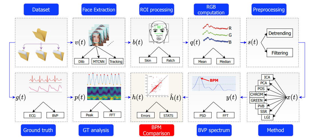
[56] M. Finžgar and P. Podržaj, “Feasibility of assessing ultra-short-term pulse rate variability from video recordings,” PeerJ, vol. 8, p. e8342, 2020.
[57] Bernau, Christoph and Riester, Markus and Boulesteix, Anne-Laure and Parmigiani, Giovanni and Huttenhower, Curtis and Waldron, Levi and Trippa, Lorenzo, “Cross-study validation for the assessment of prediction algorithms,” Bioinformatics, vol. 30, no. 12, pp. i105–i112, 2014.
[58] Nadeau, Claude and Bengio, Yoshua, “Inference for the generalization error,” in Advances in neural information processing systems, 2000, pp. 307–313.
VOLUME 4, 2016
21

This work is licensed under a Creative Commons Attribution 4.0 License. For more information, see https://creativecommons.org/licenses/by/4.0/